This section describes an example experiment using MITgcm to simulate a
baroclinic, wind and buoyancy-forced, double-gyre ocean circulation. Unlike tutorial
Barotropic Ocean Gyre, which used a Cartesian grid and a single vertical
layer, here the grid employs spherical polar coordinates with 15 vertical layers.
The configuration is similar to the double-gyre setup first solved numerically
in Cox and Bryan (1984) [CB84]: the model is configured to
represent an enclosed sector of fluid on a sphere, spanning the tropics to mid-latitudes,
\(60^{\circ} \times 60^{\circ}\) in lateral extent.
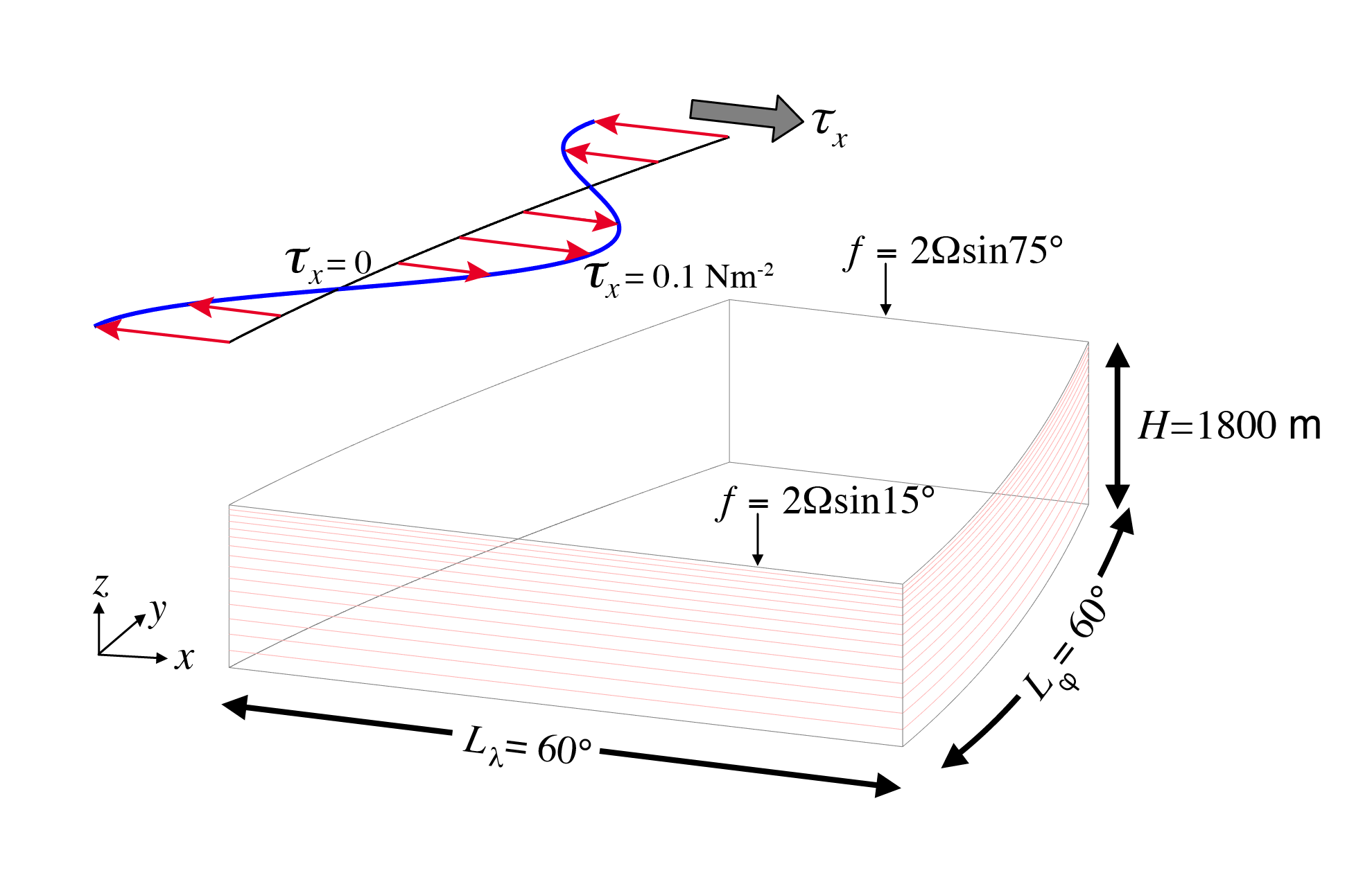
The fluid is \(1.8\) km deep and is forced by a zonal wind
stress which is constant in time, \(\tau_{\lambda}\), varying sinusoidally in the
north-south direction. The Coriolis parameter, \(f\), is defined
according to latitude \(\varphi\)
\[f(\varphi) = 2 \Omega \sin( \varphi )\]
with the rotation rate, \(\Omega\) set to \(\frac{2 \pi}{86164} \text{s}^{-1}\) (i.e., corresponding the to standard Earth rotation rate).
The sinusoidal wind-stress variations are defined according to
where \(L_{\varphi}\) is the lateral domain extent
(\(60^{\circ}\)), \(\varphi_o\) is set to \(15^{\circ} \text{N}\) and \(\tau_0\) is \(0.1 \text{ N m}^{-2}\).
Figure 4.5 summarizes the
configuration simulated. As indicated by the axes in the lower left of the figure, the
model code works internally in a locally orthogonal coordinate
\((x,y,z)\). For this experiment description the local orthogonal
model coordinate \((x,y,z)\) is synonymous with the coordinates
\((\lambda,\varphi,r)\) shown in Figure 1.20.
Initially the fluid is stratified
with a reference potential temperature profile that varies from \(\theta=30 \text{ } ^{\circ}\)C
in the surface layer to \(\theta=2 \text{ } ^{\circ}\)C in the bottom layer.
The equation of state used in this experiment is linear:
with \(\rho_{0}=999.8\,{\rm kg\,m}^{-3}\) and
\(\alpha_{\theta}=2\times10^{-4}\,{\rm K}^{-1}\).
Given the linear equation of state, in this configuration the model state variable for temperature is
equivalent to either in-situ temperature, \(T\), or potential
temperature, \(\theta\). For consistency with later examples, in
which the equation of state is non-linear, here we use the variable \(\theta\) to
represent temperature.
Figure 4.5 Schematic of simulation domain and wind-stress forcing function for baroclinic gyre numerical experiment. The domain is enclosed by solid walls.
Temperature is restored in the surface layer to a linear profile:
For this problem the implicit free surface, HPE
form of the equations (see Section 1.3.4.2; Section 2.4)
described in Marshall et al. (1997) [MHPA97] are
employed. The flow is three-dimensional with just temperature,
\(\theta\), as an active tracer.
The viscous and diffusive terms provides viscous dissipation
and a diffusive sub-grid scale closure for the momentum and temperature equations, respectively.
A wind-stress momentum forcing is added to the
momentum equation for the zonal flow, \(u\). Other terms in the
model are explicitly switched off for this experiment configuration (see
Section 4.2.3). This yields an active set of
equations solved in this configuration, written in spherical polar
coordinates as follows:
(4.15)\[p^{\prime} = g\rho_{c} \eta + \int^{0}_{z} g \rho^{\prime} dz\]
where \(u\) and \(v\) are the components of the horizontal flow
vector \(\vec{u}\) on the sphere
(\(u=\dot{\lambda},v=\dot{\varphi}\)), \(a\) is the distance from the center of the Earth,
\(\rho_c\) is a fluid density (which appears in the momentum equations,
and can be set differently than \(\rho_0\) in (4.9)),
\(A_h\) and \(A_v\) are horizontal and vertical viscosity, and
\(\kappa_h\) and \(\kappa_v\) are horizontal and vertical diffusivity, respectively.
The terms \(H\widehat{u}\) and \(H\widehat{v}\) are the components of the
vertical integral term given in equation (1.35) and explained
in more detail in Section 2.4.
However, for the problem presented here, the continuity relation
(4.13) differs from the general form
given in Section 2.4, equation (2.10)
because the source terms
\({\mathcal P}-{\mathcal E}+{\mathcal R}\) are all zero.
The forcing terms \(\mathcal{F}_u\), \(\mathcal{F}_v\), and \(\mathcal{F}_\theta\) are
applied as source terms in the model surface layer and are zero in the interior.
The windstress forcing, \({\mathcal F}_u\) and \({\mathcal F}_v\), is
applied in the zonal and meridional momentum
equations, respectively; in this configuration, \(\mathcal{F}_u = \tau_x / (\rho_c\Delta z_s)\)
(where \(\Delta z_s\) is the depth of the surface model gridcell), and
\(\mathcal{F}_v = 0\). Similarly, \(\mathcal{F}_\theta\) is applied in the temperature equation,
as given by (4.10).
In (4.15) the pressure field, \(p^{\prime}\), is separated into a barotropic
part due to variations in sea-surface height, \(\eta\), and a
hydrostatic part due to variations in density, \(\rho^{\prime}\),
integrated through the water column. Note the \(g\) in the first term on the right hand side is
MITgcm parameter gBaro whereas in the seond term \(g\) is parameter gravity;
allowing for different gravity constants here is useful, for example, if one wanted to slow down external gravity waves.
In the momentum equations, lateral and vertical boundary conditions for
the \(\nabla_{h}^{2}\) and \(\partial_z^2\) operators are specified in the
runtime configuration - see Section 4.2.3.
For temperature, the boundary condition along the bottom and sidewalls is zero-flux.
The domain is discretized with a uniform grid spacing in latitude and
longitude \(\Delta \lambda=\Delta \varphi=1^{\circ}\), so that there
are 60 active ocean grid cells in the zonal and meridional directions. As in tutorial
Barotropic Ocean Gyre, a border row of land cells surrounds the
ocean domain, so the full numerical grid size is 62\(\times\)62 in the horizontal.
The domain has 15 levels in the vertical, varying from \(\Delta z = 50\) m deep in the surface layer
to 190 m deep in the bottom layer, as shown by the faint red lines in Figure 4.5.
The internal, locally orthogonal,
model coordinate variables \(x\) and \(y\) are initialized from
the values of \(\lambda\), \(\varphi\), \(\Delta \lambda\)
and \(\Delta \varphi\) in radians according to:
\[\begin{split}\begin{aligned} x &= a\cos(\varphi)\lambda, \phantom{WWW} \Delta x = a\cos(\varphi)\Delta \lambda \\
y &= a\varphi, \phantom{WWWWWW} \Delta y = a\Delta \varphi \end{aligned}\end{split}\]
See Section 1.6.1 for additional description of spherical coordinates.
As described in Section 2.16, the time evolution of
potential temperature \(\theta\) in (4.14)
is evaluated prognostically. The centered
second-order scheme with Adams-Bashforth II time stepping described in
Section 2.16.1 is used to step forward the
temperature equation.
Prognostic terms in the momentum equations are
solved using flux form as described in Section 2.14.
The pressure forces that drive
the fluid motions, \(\partial_{\lambda} p^\prime\)
and \(\partial_{\varphi} p^\prime\), are found by
summing pressure due to surface elevation \(\eta\) and the
hydrostatic pressure, as discussed in Section 4.2.1.
The hydrostatic part of the pressure is
diagnosed explicitly by integrating density.
The sea-surface height is found by solving implicitly the 2-D (elliptic) surface pressure equation
(see Section 2.4).
The analysis in this section is similar to that discussed in
tutorial Barotropic Ocean Gyre,
albeit with some added wrinkles. In this experiment, we not only have a larger model domain extent, with greater variation
in the Coriolis parameter between the southernmost and northernmost gridpoints, but also significant variation
in the grid \(\Delta x\) spacing.
In order to choose an appropriate time step, note that our smallest gridcells (i.e., in the far north)
have \(\Delta x \approx 29\) km, which
is similar to our grid spacing in tutorial Barotropic Ocean Gyre. Thus, using the advective
CFL condition, first assuming our solution will achieve maximum horizontal advection \(|c_{\rm max}|\) ~ 1 ms-1)
we choose the same time step as in tutorial Barotropic Ocean Gyre,
\(\Delta t\) = 1200 s (= 20 minutes), resulting in \(S_{\rm adv} = 0.08\).
Also note this time step is stable for propagation of internal gravity waves:
approximating the propagation speed as \(\sqrt{g' h}\) where \(g'\) is reduced gravity (our maximum
\(\Delta \rho\) using our linear equation of state is
\(\rho_{0} \alpha_{\theta} \Delta \theta = 6\) kg/m3) and \(h\) is the upper layer depth
(we’ll assume 150 m), produces an estimated propagation speed generally less than \(|c_{\rm max}| = 3\) ms–1
(see Adcroft 1995 [Adc95] or Gill 1982 [Gil82]), thus still comfortably below the threshold.
Using our chosen value of \(\Delta t\), numerical stability for inertial oscillations using Adams-Bashforth II
(4.17)\[S_{\rm inert} = f {\Delta t} < 0.5 \text{ for stability}\]
evaluates to 0.17 for the largest \(f\) value in our domain (\(1.4\times10^{-4}\) s–1),
below the stability threshold.
To choose a horizontal Laplacian eddy viscosity \(A_{h}\), note that the largest \(\Delta x\)
value in our domain (i.e., in the south) is \(\approx 110\) km. With the Munk boundary width as follows,
in order to to have a well resolved boundary current in the subtropical gyre we will set
\(A_{h} = 5000\) m2 s–1. This results in a boundary current
resolved across two to three grid cells in the southern portion of the domain.
Given that our choice for \(A_{h}\) in this experiment is an order of magnitude larger than in
tutorial Barotropic Ocean Gyre,
let’s re-examine the stability of horizontal Laplacian friction:
evaluates to 0.057 for our smallest \(\Delta x\), which is below the stability threshold.
Note this same stability test also applies to horizontal Laplacian diffusion of tracers, with \(\kappa_{h}\) replacing
\(A_{h}\), but we will choose \(\kappa_{h} \ll A_{h}\) so this should not pose any stability issues.
Finally, stability of vertical diffusion of momentum:
Here we will choose \(A_{v} = 1\times10^{-2}\) m2 s–1,
so \(S_{lv}\) evaluates to 0.02 for our minimum \(\Delta z\),
well below the stability threshold. Note if we were to use Adams Bashforth II for diffusion of tracers
the same check would apply, with \(\kappa_{v}\) replacing \(A_{v}\). However, we will instead choose
an implicit scheme for computing vertical diffusion of tracers (see Section 4.2.3.2.1), which is unconditionally stable.
1#-- list of packages (or group of packages) to compile for this experiment:
2gfd
3diagnostics
4mnc
Here we specify which MITgcm packages we want to include in our configuration. gfd
is a pre-defined “package group” (see Using MITgcm Packages)
of standard packages necessary for most setups; it is also the default compiled packages setting
and the minimum set of packages necessary for GFD-type setups.
In addition to package group gfd we include two additional packages (individual packages, not package groups), mnc
and diagnostics. Package mnc is required
for output to be dumped in netCDF format. Package diagnostics
allows one to choose output from a extensive list of model diagnostics, and specify output frequency, with multiple time averaging or snapshot options available.
Without this package enabled, output is limited to a small number of snapshot output fields. Subsequent tutorial experiments will explore the use
of packages which expand the physical and scientific capabilities of MITgcm, e.g., such as physical parameterizations or modeling capabilities
for tracers, ice, etc., that are not compiled unless specified.
1CBOP
2C !ROUTINE: SIZE.h
3C !INTERFACE:
4C include SIZE.h
5C !DESCRIPTION: \bv
6C *==========================================================*
7C | SIZE.h Declare size of underlying computational grid.
8C *==========================================================*
9C | The design here supports a three-dimensional model grid
10C | with indices I,J and K. The three-dimensional domain
11C | is comprised of nPx*nSx blocks (or tiles) of size sNx
12C | along the first (left-most index) axis, nPy*nSy blocks
13C | of size sNy along the second axis and one block of size
14C | Nr along the vertical (third) axis.
15C | Blocks/tiles have overlap regions of size OLx and OLy
16C | along the dimensions that are subdivided.
17C *==========================================================*
18C \ev
19C
20C Voodoo numbers controlling data layout:
21C sNx :: Number of X points in tile.
22C sNy :: Number of Y points in tile.
23C OLx :: Tile overlap extent in X.
24C OLy :: Tile overlap extent in Y.
25C nSx :: Number of tiles per process in X.
26C nSy :: Number of tiles per process in Y.
27C nPx :: Number of processes to use in X.
28C nPy :: Number of processes to use in Y.
29C Nx :: Number of points in X for the full domain.
30C Ny :: Number of points in Y for the full domain.
31C Nr :: Number of points in vertical direction.
32CEOP
33 INTEGER sNx
34 INTEGER sNy
35 INTEGER OLx
36 INTEGER OLy
37 INTEGER nSx
38 INTEGER nSy
39 INTEGER nPx
40 INTEGER nPy
41 INTEGER Nx
42 INTEGER Ny
43 INTEGER Nr
44 PARAMETER (
45 & sNx = 31,
46 & sNy = 31,
47 & OLx = 2,
48 & OLy = 2,
49 & nSx = 2,
50 & nSy = 2,
51 & nPx = 1,
52 & nPy = 1,
53     &           Nx  = sNx*nSx*nPx,
54     &           Ny  = sNy*nSy*nPy,
55 & Nr = 15)
5657C MAX_OLX :: Set to the maximum overlap region size of any array
58C MAX_OLY that will be exchanged. Controls the sizing of exch
59C routine buffers.
60 INTEGER MAX_OLX
61 INTEGER MAX_OLY
62 PARAMETER ( MAX_OLX = OLx,
63 & MAX_OLY = OLy )
64
For this second tutorial, we will break the model domain into multiple tiles. Although initially we will
run the model on a single processor, a multi-tiled setup
is required when we demonstrate how to run the model using either
MPI or using multiple threads.
The following lines calculate the horizontal size of the global model domain (NOT to be edited).
Our values for SIZE.h parameters
below must multiply so that our horizontal model domain is 62\(\times\)62:
53 & Nx = sNx*nSx*nPx,
54 & Ny = sNy*nSy*nPy,
Now let’s look at all individual SIZE.h parameter settings.
Although our model domain is 62\(\times\)62, here we specify the size of a single tile to be one-half that
in both \(x\) and \(y\). Thus, the model requires four of these tiles to cover the full ocean sector domain
(see below, where we set nSx and nSy). Note that the grid
can only be subdivided into tiles in the horizontal dimensions, not in the vertical.
45     &           sNx =  31,
46     &           sNy =  31,
As in tutorial Barotropic Ocean Gyre, here we set the overlap extent of a model tile
to the value 2 in both \(x\) and \(y\). In other words, although our model tiles are sized 31\(\times\)31,
in MITgcm array storage there are an additional 2 border rows surrounding
each tile which contain model data from neighboring tiles.
Some horizontal advection schemes and other parameter and setup choices
require a larger overlap setting (see Table 2.2).
In our configuration, we are using a second-order center-differences advection scheme (the MITgcm default)
which does not requires setting a overlap beyond the MITgcm minimum 2.
47     &           OLx =   2,
48     &           OLy =   2,
These lines set parameters nSx and nSy,
the number of model tiles in the \(x\) and \(y\) directions, respectively,
which execute on a single process. Initially, we will run the model on a single core,
thus both nSx and nSy are set to 2 so that all \(2 \times 2 = 4\) tiles are integrated forward in time.
49     &           nSx =   2,
50     &           nSy =   2,
These lines set parameters nPx and nPy, the number of processes
to use in the \(x\) and \(y\) directions, respectively.
As noted, initially we will run using a single process, so for now these parameters are both set to 1.
51     &           nPx =   1,
52     &           nPy =   1,
Here we tell the model we are using 15 vertical levels.
1C Diagnostics Array Dimension
2C ---------------------------
3C ndiagMax :: maximum total number of available diagnostics
4C numlists :: maximum number of diagnostics list (in data.diagnostics)
5C numperlist :: maximum number of active diagnostics per list (data.diagnostics)
6C numLevels :: maximum number of levels to write (data.diagnostics)
7C numDiags :: maximum size of the storage array for active 2D/3D diagnostics
8C nRegions :: maximum number of regions (statistics-diagnostics)
9C sizRegMsk :: maximum size of the regional-mask (statistics-diagnostics)
10C nStats :: maximum number of statistics (e.g.: aver,min,max ...)
11C diagSt_size:: maximum size of the storage array for statistics-diagnostics
12C Note : may need to increase "numDiags" when using several 2D/3D diagnostics,
13C and "diagSt_size" (statistics-diags) since values here are deliberately small.
14 INTEGER ndiagMax
15 INTEGER numlists, numperlist, numLevels
16 INTEGER numDiags
17 INTEGER nRegions, sizRegMsk, nStats
18 INTEGER diagSt_size
19 PARAMETER( ndiagMax = 500 )
20 PARAMETER( numlists = 10, numperlist = 50, numLevels=2*Nr )
21 PARAMETER( numDiags = 20*Nr )
22 PARAMETER( nRegions = 0 , sizRegMsk = 1 , nStats = 4 )
23 PARAMETER( diagSt_size = 10*Nr )
242526CEH3 ;;; Local Variables: ***
27CEH3 ;;; mode:fortran ***
28CEH3 ;;; End: ***
In the default version /pkg/diagnostics/DIAGNOSTICS_SIZE.h the storage array for diagnostics is purposely
set quite small, in other words forcing the user to assess how many diagnostics will be computed and thus choose an appropriate
size for a storage array. In the above file we have modified the value of parameter numDiags:
21 PARAMETER( numDiags = 20*Nr )
from its default value 1*Nr, which would only allow a single 3-D diagnostic to be computed and saved, to 20*Nr,
which will permit up to some combination of up to 20 3-D diagnostics or 300 2-D diagnostic fields.
These lines set parameters viscAh and viscAr, the horizontal and vertical Laplacian viscosities respectively,
to \(5000\) m2 s–1 and \(1 \times 10^{-2}\) m2 s–1. Note the subscript \(r\)
is used for the vertical, reflecting MITgcm’s generic \(r\)-vertical coordinate capability (i.e., the model is capable of
using either a \(z\)-coordinate or a \(p\)-coordinate system).
4 viscAh=5000.,
5 viscAr=1.E-2,
These lines set parameters to specify the boundary conditions for momentum on the model domain sidewalls and bottom.
Parameter no_slip_sides is set to .TRUE., i.e., no-slip lateral boundary conditions (the default), which will yield a Munk (1950) [Mun50] western boundary solution.
Parameter no_slip_bottom is set to .FALSE., i.e., free-slip bottom boundary condition (default is true).
If instead of a Munk layer we desired a Stommel (1948) [Sto48] western boundary layer solution, we would opt for free-slip lateral boundary conditions and no-slip conditions along the bottom.
6 no_slip_sides=.TRUE.,
7 no_slip_bottom=.FALSE.,
These lines set parameters diffKhT and diffKrT,
the horizontal and vertical Laplacian temperature diffusivities respectively,
to \(1000\) m2 s–1 and \(1 \times 10^{-5}\) m2 s–1.The boundary condition on this
operator is zero-flux at all boundaries.
8 diffKhT=1000.,
9 diffKrT=1.E-5,
By default, MITgcm does not apply any parameterization to mix statically unstable columns of water. In a coarse resolution, hydrostatic
configuration, typically such a parameterization is desired. We recommend a scheme which
simply applies (presumably, large) vertical diffusivity between statically unstable grid cells in the vertical. This vertical diffusivity
is set by parameter ivdc_kappa, which here we set to \(1.0\) m2 s–1. This scheme requires that
implicitDiffusion is set to .TRUE. (see Section 2.6;
more specifically, applying a large vertical diffusivity to represent convective mixing
requires the use of an implicit
time-stepping method for vertical diffusion, rather than Adams Bashforth II).
Alternatively, a traditional convective adjustment scheme is available; this can be activated
through the cAdjFreq parameter, see Section 3.8.5.4.
10 ivdc_kappa=1.,
11 implicitDiffusion=.TRUE.,
The following parameters tell the model to use a linear equation of state.
Note a list of Nr (=15, from SIZE.h)
potential temperature values in oC is specified for parameter tRef, ordered from surface to depth.
tRef is used for two purposes here.
First, anomalies in density are computed using this reference \(\theta\), \(\theta'(x,y,z) = \theta(x,y,z) - \theta_{\rm ref}(z)\);
see use in (4.8) and (4.9).
Second, the model will use these reference temperatures for its initial state, as we are not providing a pickup file
nor specifying an initial temperature hydrographic file (in later tutorials we will demonstrate how to do so).
For each depth level the initial and reference profiles will be uniform in \(x\) and \(y\).
Note when checking static stability or computing \(N^2\), the density gradient resulting from these specified reference levels
is added to \(\partial \rho' / \partial z\) from (4.9).
Finally, we set the thermal expansion coefficient \(\alpha_{\theta}\) (tAlpha)
as used in (4.8) and (4.9), while setting
the haline contraction coefficient (sBeta) to zero (see (4.8), which omits a salinity contribution to the
linear equation of state; like tutorial Barotropic Ocean Gyre,
salinity is not included as a tracer in this very idealized model setup).
This line sets parameter \(\rho_0\) (rhoNil) to 999.8 kg/m3, the surface reference density for our linear equation of state,
i.e., the density of water at tRef(k=1). This value will also be used
as \(\rho_c\) (parameter rhoConst) in (4.11)-(4.15),
lacking a separate explicit assignment of rhoConst in data.
Note this value is the model default value for rhoNil.
16 rhoNil=999.8,
This line sets parameter gravity, the acceleration due to gravity \(g\) in (4.15), and this value will also
be used to set gBaro, the barotopic (i.e., free surface-related)
gravity parameter which we set in tutorial Barotropic Ocean Gyre.
This is the MITgcm default value.
17 gravity=9.81,
These lines set parameters which prescribe the linearized free surface formulation,
similar to tutorial Barotropic Ocean Gyre. Note
we have added parameter exactConserv, set to .TRUE.: this instructs the model to
recompute divergence after the pressure solver step, ensuring volume conservation of the free surface solution
(the model default is NOT to recompute divergence, but given the small numerical cost, we typically recommend doing so).
In tutorial Barotropic Ocean Gyre we specified a starting iteration number nIter0
and a number of time steps to integrate, nTimeSteps. Here we opt to use another approach to control run start and duration:
we set a startTime and endTime, both in units of seconds. Given a starting time of 0.0, the model starts
from rest using specified initial values of temperature (here, as previously noted, from the tRef parameter) rather than attempting
to restart from a saved checkpoint file. The specified value for endTime, 12000.0 seconds
is equivalent to 10 time steps, set for testing purposes.
To integrate over a longer, more physically relevant period of time, uncomment the endTime and monitorFreq lines
located near the end of this parameter block. Note, for simplicity, our units for these time choices assume a 360-day “year”
and 30-day “month” (although lacking a seasonal cycle in our forcing, defining a “year” is immaterial; we will demonstrate how to apply time-varying
forcings in later tutorials).
Remaining time stepping parameter choices (specifically, \(\Delta t\),
checkpoint frequency, output frequency, and monitor settings)
are described in tutorial Barotropic Ocean Gyre;
refer to the description here.
The parameter tauThetaClimRelax sets the time scale, in seconds,
for restoring potential temperature in the model’s top surface layer (see (4.10)).
Our choice here of 2,592,000 seconds is equal to 30 days.
This line sets parameter usingSphericalPolarGrid, which specifies that the simulation will use spherical polar coordinates
(and affects the interpretation of other grid coordinate parameters).
49 usingSphericalPolarGrid=.TRUE.,
These lines set the horizontal grid spacing, as vectors delX and delY
(i.e., \(\Delta x\) and \(\Delta y\) respectively), with units of degrees
as dictated by our choice usingSphericalPolarGrid.
As before, this syntax indicates that we specify 62 values in both the \(x\) and \(y\) directions, which matches the
global domain size as specified in SIZE.h.
Our ocean sector domain starts at \(0^\circ\) longitude and \(15^\circ\) N; accounting for a surrounding land
row of cells, we thus set the origin in longitude to \(-1.0^\circ\) and in latitude to \(14.0^\circ\).
Again note that our origin specifies the southern and western edges of the gridcell, not the cell center location.
Setting the origin in latitude is critical given that it affects the Coriolis parameter \(f\)
(which appears in (4.11) and (4.12)); the default value for ygOrigin is \(0.0^\circ\).
Note that setting xgOrigin is optional, given that absolute longitude does not appear in the equation discretization.
This line sets parameter delR, the vertical grid spacing in the \(z\)-coordinate (i.e., \(\Delta z\)),
to a vector of 15 depths (in meters), from 50 m in the surface layer to a bottom layer depth of 190 m. The sum of these
specified depths equals 1800 m, the full depth \(H\) of our idealized ocean sector.
Here we activate two MITgcm packages that are not included with the model by default:
package mnc (see Section 9.3) specifies that model output should be written in netCDF format,
and package diagnostics (see Section 9.1) allows user-selectable diagnostic output.
The boolean parameters set are useMNC and useDiagnostics, respectively.
Note these add-on packages also need to be specified when the model is compiled, see Section 4.2.3.1.
Apart from these two additional packages, only standard packages (i.e., those compiled in MITgcm by default) are required for this setup.
This file sets parameters which affect package pkg/mnc behavior; in fact, with pkg/mnc enabled, it is required
(many packages look for file data.«PACKAGENAME» and will terminate if not present).
By setting the parameter monitor_mnc to .FALSE.
we are specifying NOT to create separate netCDF
output files for pkg/monitor output, but rather to include this monitor output in the standard output file
(see Section 4.1.4). See Section 9.3.1.2 for a complete
listing of pkg/mnc namelist parameters and their default settings.
Unlike raw binary output, which overwrites any existing files, when using mnc output the model will create new directories if the parameters
mnc_use_outdir and mnc_outdir_str are set, as above; the model will append a 4-digit number to mnc_outdir_str,
starting at 0001, incrementing as needed if existing directories already exist.
If these parameters are NOT set, the model will terminate with an error if one attempts
to overwrite an existing .nc file (in other words, to re-run in an previous run directory,
one must delete all *.nc files before restarting). Note that our subdirectory name choice mnc_test_ is required
by MITgcm automated testing protocols, and can be changed to something more mnemonic, if desired.
In general, it is good practice to write diagnostic output into subdirectories, to keep the top run directory
less “cluttered”; some unix file systems do not respond well when very large numbers of files are produced, which can
occur in setups divided into many tiles and/or when many diagnostics are selected for output.
1# Diagnostic Package Choices
2#--------------------
3# dumpAtLast (logical): always write output at the end of simulation (default=F)
4# diag_mnc (logical): write to NetCDF files (default=useMNC)
5#--for each output-stream:
6# fileName(n) : prefix of the output file name (max 80c long) for outp.stream n
7# frequency(n):< 0 : write snap-shot output every |frequency| seconds
8# > 0 : write time-average output every frequency seconds
9# timePhase(n) : write at time = timePhase + multiple of |frequency|
10# averagingFreq : frequency (in s) for periodic averaging interval
11# averagingPhase : phase (in s) for periodic averaging interval
12# repeatCycle : number of averaging intervals in 1 cycle
13# levels(:,n) : list of levels to write to file (Notes: declared as REAL)
14# when this entry is missing, select all common levels of this list
15# fields(:,n) : list of selected diagnostics fields (8.c) in outp.stream n
16# (see "available_diagnostics.log" file for the full list of diags)
17# missing_value(n) : missing value for real-type fields in output file "n"
18# fileFlags(n) : specific code (8c string) for output file "n"
19#--------------------
20 &DIAGNOSTICS_LIST
21  fields(1:3,1)  = 'ETAN    ','TRELAX  ','MXLDEPTH',
22  fileName(1) = 'surfDiag',
23  frequency(1) = 31104000.,
2425 fields(1:5,2) = 'THETA ','PHIHYD ',
26 'UVEL ','VVEL ','WVEL ',
27# did not specify levels => all levels are selected
28 fileName(2) = 'dynDiag',
29 frequency(2) = 31104000.,
30 &
3132#--------------------
33# Parameter for Diagnostics of per level statistics:
34#--------------------
35# diagSt_mnc (logical): write stat-diags to NetCDF files (default=diag_mnc)
36# diagSt_regMaskFile : file containing the region-mask to read-in
37# nSetRegMskFile : number of region-mask sets within the region-mask file
38# set_regMask(i) : region-mask set-index that identifies the region "i"
39# val_regMask(i) : region "i" identifier value in the region mask
40#--for each output-stream:
41# stat_fName(n) : prefix of the output file name (max 80c long) for outp.stream n
42# stat_freq(n):< 0 : write snap-shot output every |stat_freq| seconds
43# > 0 : write time-average output every stat_freq seconds
44# stat_phase(n) : write at time = stat_phase + multiple of |stat_freq|
45# stat_region(:,n) : list of "regions" (default: 1 region only=global)
46# stat_fields(:,n) : list of selected diagnostics fields (8.c) in outp.stream n
47# (see "available_diagnostics.log" file for the full list of diags)
48#--------------------
49 &DIAG_STATIS_PARMS
50 stat_fields(1:2,1) = 'THETA ','TRELAX ',
51 stat_fName(1) = 'dynStDiag',
52 stat_freq(1) = 2592000.,
53 &
In this section we specify what diagnostics we want to compute, how frequently to compute them, and the name of output files.
Multiple diagnostic fields can be grouped into individual files (i.e., an individual output file here is associated with a ‘list’ of diagnostics).
The above lines tell MITgcm that our first list will consist of three diagnostic variables:
ETAN - the linearized free surface height (m)
TRELAX - the heat flux entering the ocean due to surface temperature relaxation (W/m2)
MXLDEPTH - the depth of the mixed layer (m), as defined here by a given magnitude decrease
in density from the surface (we’ll use the model default for \(\Delta \rho\))
Note that all these diagnostic
fields are 2-D output. 2-D and 3-D diagnostics CANNOT be mixed in a diagnostics list.
These variables are specified in parameter fields: the first index is specified as 1:«NUMBER_OF_DIAGS», the second index
designates this for diagnostics list 1. Next, the output filename for diagnostics list 1 is specified in variable fileName. Finally,
for this list we specify variable frequency to provide time-averaged output every 31,104,000 seconds,
i.e., once per year. Had we entered
a negative value for frequency, MITgcm would have instead written snapshot data at this interval.
Next, we set up a second diagnostics list for several 3-D diagnostics.
25  fields(1:5,2)  = 'THETA   ','PHIHYD  ',
26                   'UVEL    ','VVEL    ','WVEL    ',
27# did not specify levels => all levels are selected
28   fileName(2) = 'dynDiag',
29  frequency(2) = 31104000.,
UVEL, VVEL, WVEL - the zonal, meridional, and vertical velocity components respectively (m/s)
Here we did not specify parameter levels, so all depth levels will be included in the output.
An example of syntax to limit which depths are output is levels(1:5,2)=1.,2.,3.,, which would dump just the top three levels.
We again specify an output file name via parameter fileName, and specify a time-average period of one year
through parameter frequency.
DIAG_STATIS_PARMS - Diagnostic Per Level Statistics
It is also possible to request output statistics averaged for global mean and by level average (for 3-D diagnostics) over the full domain,
and/or for a pre-defined \((x,y)\) region of the model grid. The statistics computed for each diagnostic are as follows:
(area weighted) mean (in both space and time, if time-averaged frequency is selected)
(area weighted) standard deviation
minimum value
maximum value
volume of the area used in the calculation (multiplied by the number of time steps if time-averaged).
While these statistics could in theory also be calculated (by the user) from 2-D and 3-D DIAGNOSTICS_LIST output, the advantage
is that much higher frequency statistical output can be achieved without filling up copious amounts of disk space.
The syntax here is analogous with DIAGNOSTICS_LIST namelist parameters, except the parameter names begin with stat
(here, stat_fields, stat_fName, stat_freq). Frequency can be set to snapshot or time-averaged output,
and multiple lists of diagnostics (i.e., separate output files) can be specified. The only major difference from
DIAGNOSTICS_LIST syntax is that 2-D and 3-D diagnostics can be mixed in a list.
As noted, it is possible to select limited horizontal regions of interest, in addition to the full domain calculation.
 1# Example "eedata" file
 2# Lines beginning "#" are comments
 3#  nTx      :: No. threads per process in X
 4#  nTy      :: No. threads per process in Y
 5# debugMode :: print debug msg (sequence of S/R calls)
 6 &EEPARMS
 7 nTx=1,
 8 nTy=1,
 9 &
10# Note: Some systems use & as the namelist terminator (as shown here).
11#       Other systems use a / character.
As shown, this file is configured for a single-threaded run, but will be modified later in this tutorial for a multi-threaded setup
(Section 4.2.6).
To build and run the model on a single processor, follow the procedure outlined in Section 4.1.4.
To run the model for a longer period (i.e., to obtain a reasonable solution; for testing purposes,
by default the model is set to run only a few time steps) uncomment the lines in data which specify
larger numbers for parameters endTime and monitorFreq. This will run the model for 100 years, which
will likely take several hours on a single processor (depending on your computer specs); below we also give instructions for running the model
in parallel either using MPI
or multi-threaded (OpenMP), which
will cut down run time significantly.
As in tutorial Barotropic Ocean Gyre, standard output is produced (redirected into
file output.txt as specified in Section 4.1.4); like before, this file
includes model startup information, parameters, etc. (see Section 4.1.4.1).
And because we set monitor_mnc=.FALSE. in data.mnc,
our standard output file will include all monitor statistics output. Note monitor statistics and cg2d
information are evaluated over the global domain, despite the bifurcation of the grid into four separate tiles.
As before, the file STDERR.0000 will contain a log of any run-time errors.
With pkg/mnc compiled and activated in data.pkg, other output is
in netCDF format: grid information,
snapshot output specified in data, diagnostics output specified in data.diagnostics
and separate files containing hydrostatic pressure data (see below).
There are two notable differences from standard binary output. Recall that we specified
that the grid was subdivided into four separate tiles (in SIZE.h);
instead of a .XXX.YYY. file naming scheme for different tiles (as discussed here),
with pkg/nmc the file names contain .t«nnn». where «nnn» is the
tile number. Secondly, model data from multiple
time snapshots (or periods) is included in a single file. Although an iteration
number is still part of the file name (here, 0000000000),
this is the iteration number at the start of the run (instead of
marking the specific iteration number for the data contained in the file, as the case
for standard binary output). Note that if you dump data frequently, standard binary can produce
huge quantities of separate files, whereas using netCDF
will greatly reduce the number of files. On the other hand, the
netCDF files created can instead become quite large.
To more easily process and plot our results as a single array over the full domain,
we will first reassemble the individual tiles into new netCDF format global data files.
To accomplish this, we will make use of utility script utils/python/MITgcmutils/scripts/gluemncbig.
From the output run (top) directory, type:
For help using this utility, type gluemncbig--help (note, this utility requires python).
The files grid.nc, state.nc, etc. are concatenated from the separate t001, t002, t003, t004 files
into global grid files of horizontal dimension 62\(\times\)62. gluemncbig is a fairly intelligent script, and by inserting the wildcards
in the path/filename specification, it will grab the most recent run (in case you have started up runs multiple times in this directory,
thus having mnc_test_0001, mnc_test_0002, etc. directories present; see Section 4.2.3.2.3).
Note that the last line above is simply making
a link to a file in the mnc_test_0001 output subdirectory; this is the statistical-dynamical diagnostics
output, which is already assembled over the global domain (and also note here we are required to be specific which mnc_test_ directory to link from).
For convenience we simply place the link at the top level
of the run directory, where the other assembled .nc files are saved by gluemncbig.
Let’s proceed through the netcdf output that is produced.
grid.nc - includes all the model grid variables used by MITgcm.
This includes the grid cell center points and separation (XC, YC, dxC, dyC),
corner point locations and separation (XG, YG, dxG, dyG),
the separation between velocity points (dyU, dxV),
vertical coordinate location and separation (RC, RF, drC, drF),
grid cell areas (rA, rAw, rAs, rAz),
and bathymetry information (Depth, HFacC, HFacW, HFacS).
See Section 2.11 for definitions and description of the C grid staggering of these variables.
There are also grid variables in vector form that are not used in the MITgcm source code
(X, Y, Xp1, Yp1, Z, Zp1, Zu, Zl); see description in grid.nc. The variables named p1 include an additional data point
and are dimensioned +1 larger than the standard array size; for example, Xp1 is the longitude of the gridcell left corner, and
includes an extra data point for the last gridcell’s right corner longitude.
state.nc - includes snapshots of state variables U, V, W, Temp, S, and Eta
at model times T in seconds (variable iter(T) stores the model iteration corresponding with these model times).
Also included are vector forms of grid variables X, Y, Z, Xp1, Yp1, and Zl.
As mentioned, in model output-by-tile files, e.g., state.0000000000.t001.nc, the iteration number 0000000000 is the parameter nIter0 for the model run
(recall, we initialized our model with nIter0 =0).
Snapshots of model state are written for model iterations 0, 25920, 51840, …
according to our data file parameter choice dumpFreq (dumpFreq/deltaT = 25920).
surfDiag.nc - includes output diagnostics as specified from list 1 in
data.diagnostics.
Here we specified that list 1 include 2-D diagnostics ETAN, TRELAX, and MXLDEPTH.
Also includes an array of model times corresponding to the end of the time-average period, the iteration
number corresponding to these model times, and vector forms of grid variables which describe these data.
A Z index is included in the output arrays, even though
its dimension is one (given that this list contains only 2-D fields).
dynDiag.nc - similar to surfDiag.nc except this file contains the time-averaged 3-D diagnostics
we specified in list 2 of data.diagnostics:
THETA, PHIHYD, UVEL, VVEL, WVEL.
dynStDiag.nc - includes output statistical-dynamical diagnostics as specified in the DIAG_STATIS_PARMS section of
data.diagnostics. Like surfDiag.nc it also
includes an array of model times and corresponding iteration numbers for each time-average period end. Output variables are 3-D:
(time, region, depth). In data.diagnostics,
we have not defined any additional regions (and by default only global output is produced, “region 1”). Depth-integrated statistics
are computed (in which case the depth subscript has a range of one element; this is also the case for surface diagnostics such as TRELAX),
but output is also tabulated at each depth for some variables (i.e., the depth subscript will range from 1 to Nr).
phiHyd.nc, phiHydLow.nc - these files contain a snapshot 3-D field of hydrostatic
pressure potential anomaly (\(p'/\rho_c\), see Section 1.3.6)
and a snapshot 2-D field of bottom hydrostatic pressure potential anomaly, respectively.
These are technically not MITgcm state variables, as they are computed during the time step
(normal snapshot state variables are dumped after the time step),
ergo they are not included in file state.nc. Like state.nc output however
these fields are written at interval according to
dumpFreq, except are not written out at time nIter0 (i.e., have one time
record fewer than state.nc). Also note when writing standard binary output, these filenames begin as PH and PHL respectively.
The hydrostatic pressure potential anomaly \(\phi'\) is computed as follows:
\[\phi' = \frac{1}{\rho_c} \left( \rho_c g \eta + \int_{z}^{0} (\rho - \rho_0) g dz \right)\]
following (4.8), (4.9) and (4.15). Note that with the linear free surface approximation,
the contribution of the free surface position \(\eta\) to \(\phi'\) involves the constant density \(\rho_c\)
and not the density anomaly \(\rho'\), in contrast with contributions from below \(z=0\).
Several additional files are output in standard binary format. These are:
RhoRef.data,RhoRef.meta - this is a 1-D (k=1…Nr) array of reference density, defined as:
PHrefC.data,PHrefC.meta,PHrefF.data,PHrefF.meta - these are 1-D (k=1…Nr for PHrefC and
k=1…Nr+1 for PHrefF) arrays containing a reference
hydrostatic “pressure potential” \(\phi = p/\rho_c\) (see Section 1.3.6).
Using a linear equation of state, PHrefC is simply \(\frac{\rho_c g |z|}{\rho_c}\),
with output computed at the midpoint of each vertical cell, whereas PHrefF
is computed at the surface and bottom of each vertical cell.
Note that these quantities are not especially useful when using a linear equation of state
(to compute the full hydrostatic pressure potential, one would use RhoRef and
integrate downward, and add phiHyd, rather than use these fields),
but are of greater utility using a non-linear equation of state.
pickup.ckptA.001.001.data, pickup.ckptA.001.001.meta, pickup.0000518400.001.001.data, pickup.0000518400.001.001.meta etc. - as
described in detail in tutorial Barotropic Gyre,
these are temporary and permanent checkpoint files, output in binary format. Note that separate checkpoint files are written for each model tile.
And finally, because we are using the diagnostics package, upon startup the file available_diagnostics.log
will be generated. This (plain text) file contains a list of all diagnostics available for output in this setup, including a description of each diagnostic and its units,
and the number of levels for which the diagnostic is available (i.e., 2-D or 3-D field). This list of available diagnostics will change based
on what packages are included in the setup. For example, if your setup includes a seaice package, many seaice diagnostics
will be listed in available_diagnostics.log that are not available for the tutorial Baroclinic Gyre setup.
% ../../../tools/genmake2 -mods ../code -mpi -of=«/PATH/TO/OPTFILE»
% make depend
% make
Note we have added the option -mpi to the genmake2 command that generates the makefile.
A successful build requires MPI libraries installed on your system, and you may need to add to your $PATH environment variable
and/or set environment variable $MPI_INC_DIR (for more details, see Section 3.5.4). If there is a problem
finding MPI libraries, genmake2 output will complain.
Next, we we change nPx and nPy so that we use two processes in each dimension, for a total of \(2*2 = 4\) processes.
Effectively, we have subdivided the model grid into four separate tiles, and the model equations are solved in parallel on four separate processes
(presumably, on a unique physical processor or core). Because of the overlap regions
(i.e., gridpoints along the tile edges are duplicated in two or more tiles), and limitations
in the transfer speed of data between processes, the model will not run 4\(\times\) faster, but should be at least 2-3\(\times\) faster than running
on a single process.
51     &           nPx =   2,
52     &           nPy =   2,
Finally, to run the model (from your run directory), using four processes running in parallel:
% mpirun -np 4 ../build_mpi/mitgcmuv
On some systems the MPI
run command (and the subsequent command-line option -np) might be something other than mpirun; ask your local system administrator.
When using a large HPC cluster,
prior steps might be required to allocate four processor cores to your job, and/or it might be necessary to
write this command within a batch scheduler script; again, check with your local system documentation or system administrator.
If four cores are not available when you execute the above mpirun command, an error will occur.
When running in parallel, pkg/mnc output will create separate output subdirectories for each
process, assuming option mnc_use_outdir
is set to TRUE (here, by specifying -np4 four directories will be created, one for each
tile – mnc_test_00001 through mnc_test_00004 – the first time
the model is run). The (global) statistical-dynamical diagnostics output file will be written in only the first of these directories.
The gluemncbig steps outlined above remain unchanged (if in doubt, one can always
tell gluemncbig which specific directories to read,
e.g., in bash mnc_test_{0009..0012} will grab only directories 0009, 0010, 0011, 0012).
Also note it is no longer necessary to redirect standard output
to a file such as output.txt; rather, separate STDOUT.xxxx and STDERR.xxxx
files are created by each process, where xxxx is the process number (starting from 0000).
Other than some additional MPI-related information,
the standard output content is similar to that from the single-process run.
To run multi-threaded (using shared memory, OpenMP),
the original SIZE.h file is used.
In our example, for compatibility with MITgcm testing protocols, we will
run using two separate threads, but the user should feel free to experiment using four threads if their local machine contains four cores.
Like the previous section we must first re-compile the executable from scratch,
using a special command line option (for this configuration, -omp). However it is not necessary to specify
how many threads at compile-time (unlike MPI, which requires specific processor count
information to be set in SIZE.h).
Create and navigate into a new build directory build_openmp and type:
% ../../../tools/genmake2 -mods ../code -omp -of=«/PATH/TO/OPTFILE»
% make depend
% make
In a run directory, overwrite the contents of eedata with file
verification/tutorial_baroclinic_gyre/input/eedata.mth. The parameter nTy is changed; we now specify to
use two threads across the \(y\)-domain. Since our model domain is subdivided into four tiles, each thread will now
integrate two tiles in the \(x\)-domain. Alternatively, to run a multi-threaded example using four threads, both lines should be set to 2.
8 nTx=1,
9 nTy=2,
To run the model, we first need to set two environment variables, before invoking the executable:
Your system’s environment variables may differ from above;
see Section 3.6.2 and/or ask your system administrator
(also note, above is bash shell syntax;
different syntax is required for C shell). The important point to note is that
we must tell the operating system environment how many threads will be used, prior to running the executable.
The total number of threads set in OMP_NUM_THREADS must match nTx * nTy as specified in file eedata.
Moreover, the model domain must be subdivided into sufficient number of tiles in SIZE.h
through the choices of nSx and nSy: the number of tiles (nSx * nSy) must be equal to or greater than the number of threads.
More specifically, nSx must be equal to or an integer multiple of nTx, and nSy must be equal to or an integer multiple of nTy.
Also note that at this time, pkg/mnc is automatically disabled for multi-threaded setups, so output
is dumped in standard binary format (i.e., using pkg/msdio). You will receive a gentle warning message if you run
this multi-threaded setup and keep useMNC set to .TRUE. in data.pkg.
The full filenames for grid variables (e.g., XC, YC, etc.), snapshot output (e.g., Eta, T, PHL)
and pkg/diagnostics output (e.g., surfDiag, oceStDiag, etc.) include a suffix
that contains the time iteration number and tile identification (tile 001 includes .001.001 in the filename,
tile 002 .002.001, tile 003 .001.002, and tile 004 .002.002).
Unfortunately there is no analogous script
to utils/python/MITgcmutils/scripts/gluemncbig to concatenate raw binary files, but it is relatively straightforward
to do so in matlab (reading in files using utils/matlab/rdmds.m), or equally simple in python – or, one could simply set
globalFiles to .TRUE. and the model will output global files for you (note, this global option is not available for pkg/mnc output).
One additional difference between pkg/msdio and
pkg/mnc is that Diagnostics Per Level Statistics are written in plain text, not binary, with pkg/msdio.
In this section, we will examine details of the model solution,
using monthly and annual mean time average data provided in diagnostics files dynStDiag.nc, dynDiag.nc, and surfDiag.nc.
See companion matlab
or python
(or python using xarray)
script which shows the code to read output netCDF files
and create figures shown in this section.
Our ocean sector model is forced mechanically by wind stress and thermodynamically
though temperature relaxation at the surface. As such,
we expect our solution to not only exhibit wind-driven gyres in the upper layers,
but also include a deep, overturning circulation. Our focus in this section
will be on the former; this component of the solution equilibrates on a time scale of decades,
more or less, whereas the deep cell depends on a slower, diffusive timescale.
We will begin by examining some of our Diagnostics Per Level Statistics output, to assess
how close we are to equilibration at different ocean model levels. Recall we’ve requested
these statistics to be computed monthly.
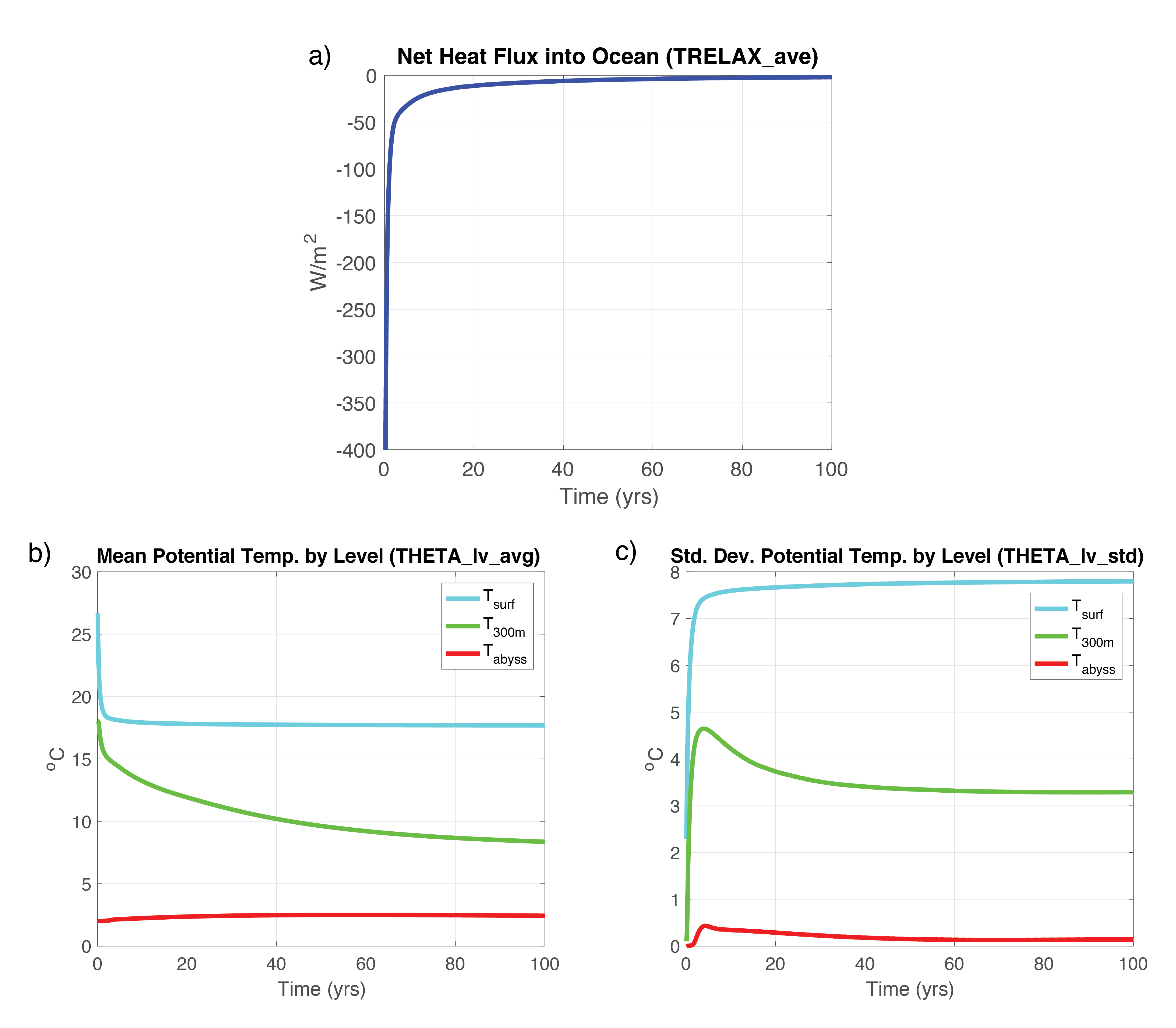
Load diagnostics TRELAX_ave, THETA_lv_avg, and THETA_lv_std from file dynStDiag.nc.
In Figure 4.6a
we plot the global model surface mean heat flux (TRELAX_ave) as a function of time.
At the beginning of the run,
we observe that the ocean is cooling dramatically; this is mainly because our ocean surface layer is
initialized to a uniform \(30^{\circ}\) C (as specified here), which results in
very strong relaxation initially in the northern portion of ocean model, where the
restoring temperature is just above \(0^{\circ}\) C.
(As an aside comment, such large initialization shocks are often best avoided
if possible, as they may cause model instability, which
may necessitate smaller time steps at model onset and/or more realistic initial conditions.)
However, this initial burst of cooling quickly diminishes over the first decade
of integration, as the surface layer approaches temperature values close to the specified profile;
see Figure 4.6b
where the mean temperature at surface, thermocline, and abyssal depth are plotted as a function of time.
Note that while the total heat flux shows that the global heat content is slowly decreasing,
even after 100 years, the temperature of the deepest water is slowly warming.
In Figure 4.6c we plot standard deviation of temperature
(by level) over time. Given that each level is initialized at uniform temperature,
initially the standard deviation is zero, but should tend to level off at some non-zero
value over time, as the solution at each depth equilibrates.
Not surprisingly, the largest gradients in temperature exist at the surface, whereas in the
abyss the differences in temperature are quite small.
In summary, we conclude that while the surface appears to approach equilibrium rapidly,
even after 100 years there are changes occurring in deep circulation, presumably related
to the meridional overturning circulation.
We leave it as an exercise to the reader to
integrate the solution further and/or examine and calculate the meridional overturning circulation strength over time.
Figure 4.6 a) Surface heat flux due to temperature restoring, negative values indicate heat flux out of the ocean;
b) and c) potential temperature mean and standard deviation by level, respectively.
Next, let’s examine the effect of wind stress on the ocean’s upper layers.
Given the orientation of the wind stress and its variation over a full sine wave as shown in Figure 4.5
(crudely mimicking easterlies in the tropics, mid-latitude westerlies, and polar easterlies),
we anticipate a double-gyre solution, with a subtropical gyre and a subpolar gyre.
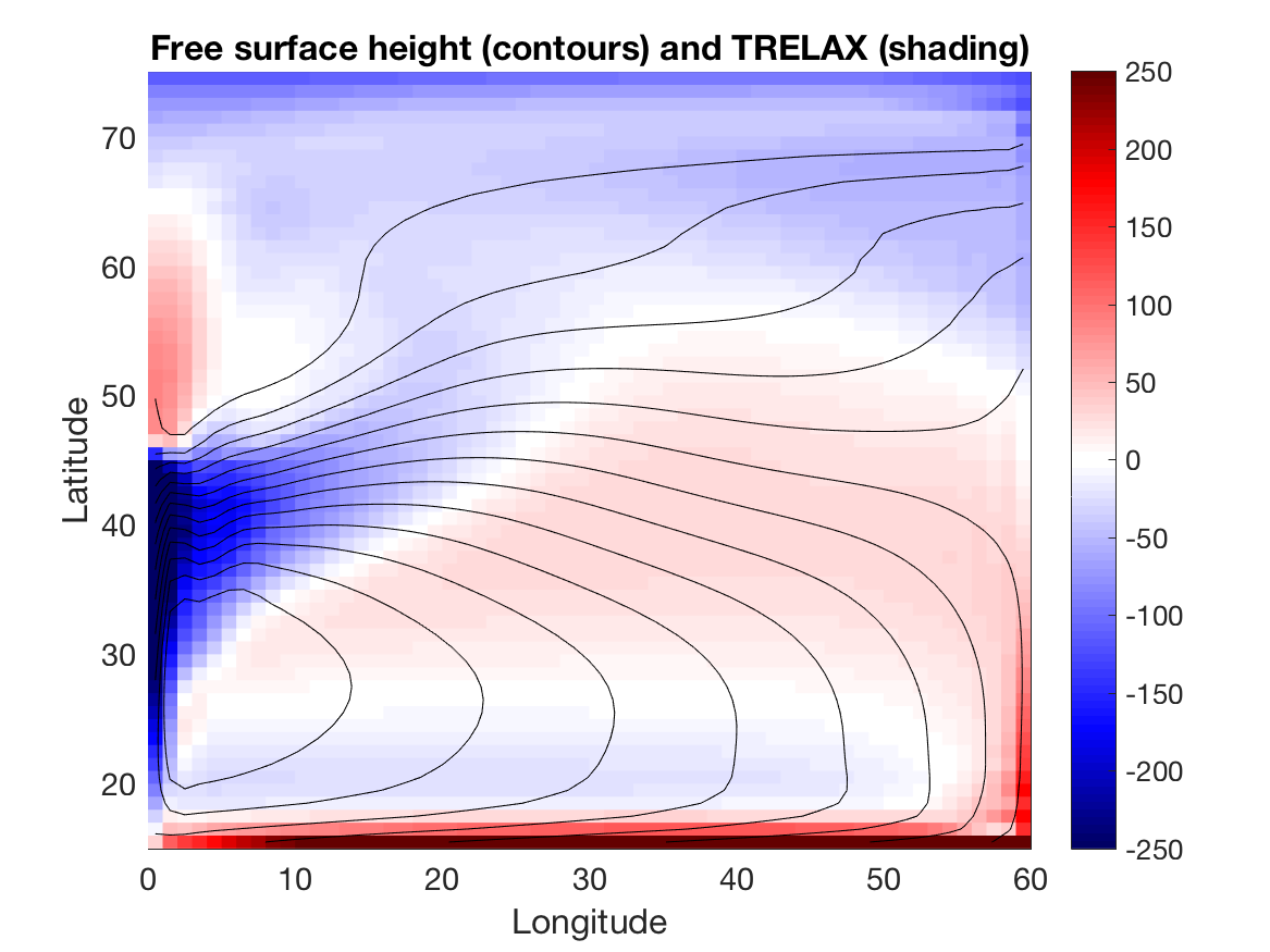
Let’s begin by examining the free surface solution (load diagnostics ETAN and TRELAX from file surfDiag.nc).
In Figure 4.7 we show contours of free surface height
(ETAN; this is what we plotted in our barotropic gyre tutorial solution)
overlaying a 2-D color plot of TRELAX
(blue is where heat is released from the ocean, red where heat enters the ocean), averaged over year 100.
Note that a subtropical gyre is readily apparent, as suggested by geostropic currents in balance with
the free surface elevation (not shown, but the reader is encouraged to load diagnostics UVEL and VVEL
and plot the circulation at various levels). Heat is entering the ocean mainly along the southern boundary,
where upwelling of cold water is occurring, but also along the boundary current between \(50^{\circ}\)N and \(65^{\circ}\)N, where we
would expect southward flow (i.e., advecting water that is colder than the local restoring temperature).
Heat is exiting the ocean where the western boundary current transports warm water northward,
before turning eastward into the basin
at \(40^{\circ}\)N, and also weakly throughout the higher latitude bands,
where deeper mixed layers occur (not shown, but variations in mixed layer
depth can be easily visualized by loading diagnostic MXLDEPTH).
Figure 4.7 Contours of free surface height (m) averaged over year 100; shading is surface heat flux due to
temperature restoring (W/m2), blue indicating cooling.
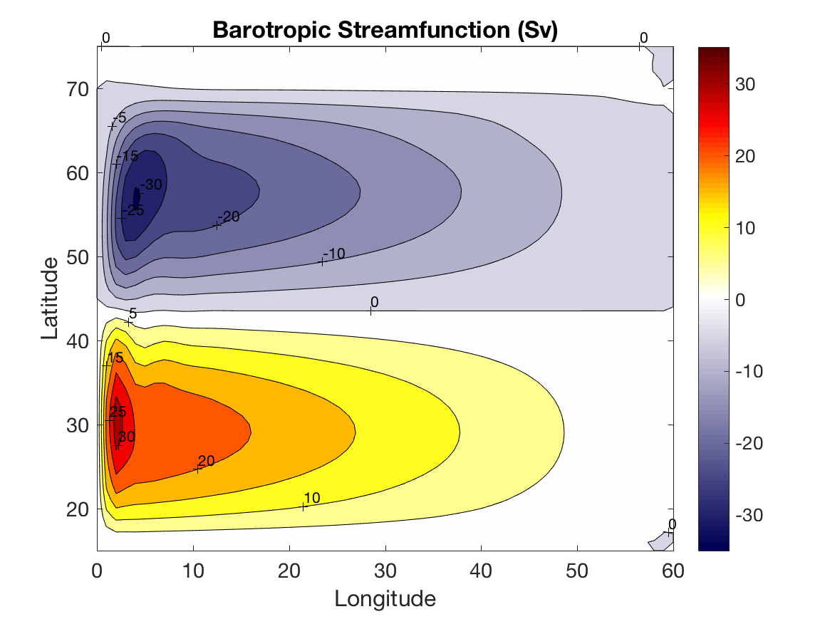
So what happened to our model solution subpolar gyre? Let’s compute depth-integrated velocity \(U_{\rm bt}, V_{\rm bt}\)
(units: m2 s-1) and use it calculate the barotropic transport streamfunction:
Compute \(U_{\rm bt}\) by summing the diagnostic UVEL multiplied by gridcell depth
(grid.nc variable drF, i.e.,
the separation between gridcell faces in the vertical). Now do a cumulative sum of
\(-U_{\rm bt}\) times the gridcell spacing the in the \(y\) direction (you
will need to load grid.nc variable dyG, the separation between gridcell faces in \(y\)).
A plot of the resulting \(\Psi\) field is shown in Figure 4.8.
Note one could also cumulative sum \(V_{\rm bt}\) times the grid spacing in the \(x\)-direction and obtain a similar result.
Figure 4.8 Barotropic streamfunction (Sv) as computed over year 100.
When velocities are integrated over depth, the subpolar gyre is readily apparent,
as might be expected given our wind stress forcing profile. The pattern in Figure 4.8 in fact resembles
the double-gyre free surface solution we observed in Figure 4.4
from tutorial Barotropic Ocean Gyre, when our model grid was only a single layer in the vertical.
Is the magnitude of \(\Psi\)
we obtain in our solution reasonable? To check this, consider the Sverdrup transport:
If we plug in a typical mid-latitude value for \(\beta\) (\(2 \times 10^{-11}\) m-1 s-1)
and note that \(\tau\) varies by \(0.1\) Nm —2 over \(15^{\circ}\) latitude,
and multiply by the width of our ocean sector, we obtain an estimate of approximately 20 Sv.
This estimate agrees reasonably well with the strength of the circulation in Figure 4.8.
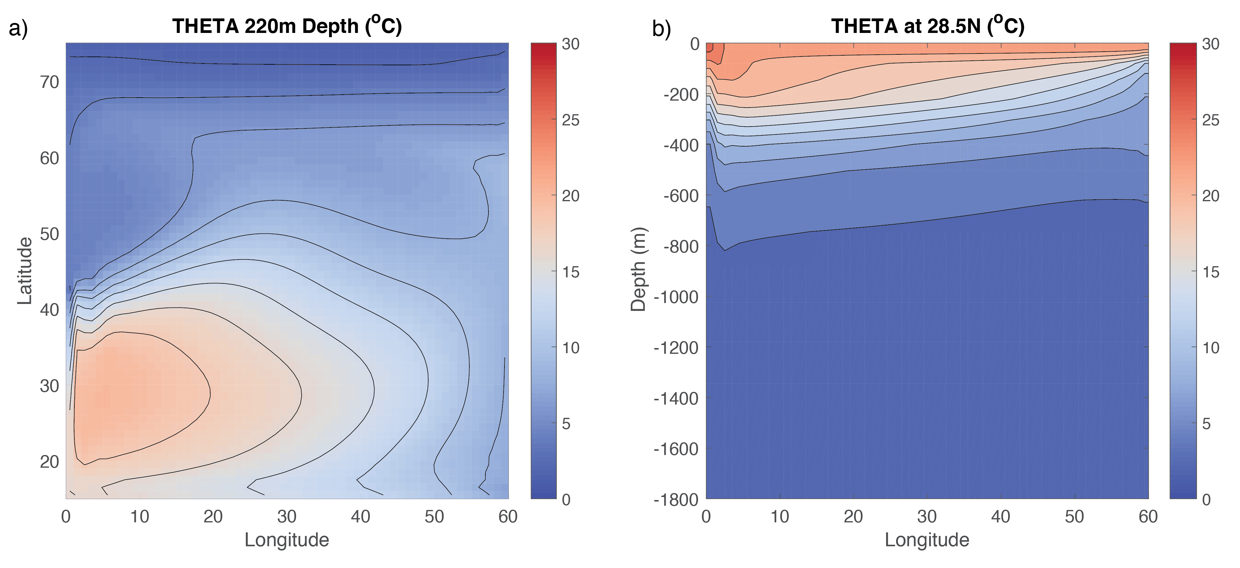
Finally, let’s examine the model solution potential temperature field averaged over year 100.
Read in diagnostic THETA from the file dynDiag.nc. Figure 4.9a shows a plan view of temperature
at 220 m depth (vertical level k=4). Figure 4.9b shows a slice in the \(xz\) plane at \(28.5^{\circ}\)N
(\(y\)-dimension j=15), through the center of the subtropical gyre.
Figure 4.9 Contour plot of potential temperature at year 100 a) at a depth of 220 m and b) through a section at \(28.5^{\circ}\)N. Contour interval is 2K.
The dynamics of the subtropical gyre are governed by
Ventilated Thermocline Theory (see, for example, Pedlosky (1996) [Ped96] or
Vallis (2017) [Val17]). Note the presence of warm “mode water” on the western side of the basin;
the contours of the warm water in the southern half of the sector crudely align with the free surface
heights we observed in Figure 4.8. In Figure 4.9b note
the presence of a thermocline, i.e., the bunching up of the contours
between 200 m and 400 m depth, with weak stratification below the thermocline.
What sets the penetration depth of the subtropical gyre? Following a simple advective scaling argument
(see Vallis (2017) [Val17] or Cushman-Roisin and Beckers (2011) [CRB11];
this scaling is obtained via thermal wind and the linearized barotropic vorticity equation),
the depth of the thermocline \(h\) should scale as:
where \(w_{\rm Ek}\) is a representive value for Ekman pumping, \(\Delta b = g \rho' / \rho_0\)
is the variation in buoyancy across the gyre,
and \(L_x\) and \(L_y\) are length scales in the
\(x\) and \(y\) directions, respectively.
Plugging in applicable values at \(30^{\circ}\)N,
we obtain an estimate for \(h\) of 200 m, which agrees quite well with that observed in Figure 4.9b.