Automatic differentiation (AD), also referred to as algorithmic (or,
more loosely, computational) differentiation, involves automatically
deriving code to calculate partial derivatives from an existing fully
non-linear prognostic code (see Griewank and Walther, 2008 [GW08]).
A software
tool is used that parses and transforms source files according to a set
of linguistic and mathematical rules. AD tools are like source-to-source
translators in that they parse a program code as input and produce a new
program code as output (we restrict our discussion to source-to-source
tools, ignoring operator-overloading tools). However, unlike a pure
source-to-source translation, the output program represents a new
algorithm, such as the evaluation of the Jacobian, the Hessian, or
higher derivative operators. In principle, a variety of derived
algorithms can be generated automatically in this way.
MITgcm has been adapted for use with the Tangent linear and Adjoint
Model Compiler (TAMC) and its successor TAF (Transformation of
Algorithms in Fortran), developed by Ralf Giering
(Giering and Kaminski, 1998 [GK98], Giering, 2000
[Gie00]). The
first application of the adjoint of MITgcm for sensitivity studies was
published by Marotzke et al. (1999) [MGZ+99].
Stammer et al. (1997, 2002) [SWG+97][SWG+02] use MITgcm and its adjoint
for ocean state estimation studies. In the following we shall refer to
TAMC and TAF synonymously, except were explicitly stated otherwise.
As of mid-2007 we are also able to generate fairly efficient adjoint
code of the MITgcm using a new, open-source AD tool, called OpenAD (see
Naumann, 2006 [NUH+06] and Utke et al., 2008 [UNF+08]).
This enables us for the
first time to compare adjoint models generated from different AD tools,
providing an additional accuracy check, complementary to
finite-difference gradient checks. OpenAD and its application to MITgcm
is described in detail in Section 7.5.
The AD tool exploits the chain rule for computing the first derivative
of a function with respect to a set of input variables. Treating a given
forward code as a composition of operations – each line representing a
compositional element, the chain rule is rigorously applied to the code,
line by line. The resulting tangent linear or adjoint code, then, may be
thought of as the composition in forward or reverse order, respectively,
of the Jacobian matrices of the forward code’s compositional elements.
Let \(\cal{M}\) be a general nonlinear, model, i.e., a mapping from
the \(m\)-dimensional space \(U \subset \mathbb{R}^m\) of input
variables \(\vec{u}=(u_1,\ldots,u_m)\) (model parameters, initial
conditions, boundary conditions such as forcing functions) to the
\(n\)-dimensional space \(V \subset \mathbb{R}^n\) of model output
variable \(\vec{v}=(v_1,\ldots,v_n)\) (model state, model
diagnostics, objective function, …) under consideration:
The vectors \(\vec{u} \in U\) and \(\vec{v} \in V\) may be
represented with respect to some given basis vectors
\({\rm span} (U) = \{ {\vec{e}_i} \}_{i = 1, \ldots , m}\) and
\({\rm span} (V) = \{ {\vec{f}_j} \}_{j = 1, \ldots , n}\) as
Consider a perturbation to the input variables \(\delta \vec{u}\)
(typically a single component
\(\delta \vec{u} = \delta u_{i} \, {\vec{e}_{i}}\)). Their effect on
the output may be obtained via the linear approximation of the model
\({\cal M}\) in terms of its Jacobian matrix \(M\), evaluated
in the point \(u^{(0)}\) according to
(7.2)\[\delta \vec{v} \, = \, M |_{\vec{u}^{(0)}} \, \delta \vec{u}\]
with resulting output perturbation \(\delta \vec{v}\). In
components
\(M_{j i} \, = \, \partial {\cal M}_{j} / \partial u_{i}\), it
reads
(7.2) is the tangent linear model (TLM). In contrast
to the full nonlinear model \({\cal M}\), the operator \(M\)
is just a matrix which can readily be used to find the forward
sensitivity of \(\vec{v}\) to perturbations in \(u\), but if
there are very many input variables \((\gg O(10^{6})\) for
large-scale oceanographic application), it quickly becomes prohibitive
to proceed directly as in (7.2), if the impact of each
component \({\bf e_{i}}\) is to be assessed.
Let us consider the special case of a scalar objective function
\({\cal J}(\vec{v})\) of the model output (e.g., the total meridional
heat transport, the total uptake of CO2 in the Southern Ocean
over a time interval, or a measure of some model-to-data misfit)
can be expressed in both bases of \(\vec{u}\) and
\(\vec{v}\) with respect to their corresponding inner product
\(\left\langle \,\, , \,\, \right\rangle\)
(note, that the gradient \(\nabla f\) is a co-vector, therefore
its transpose is required in the above inner product). Then, using the
representation of \(\delta {\cal J} =
\left\langle \, \nabla _{v}{\cal J}^T \, , \, \delta \vec{v} \, \right\rangle\),
the definition of an adjoint operator \(A^{\ast}\) of a given
operator \(A\),
With the identity (7.5), we then find that the gradient
\(\nabla _{u}{\cal J}\) can be readily inferred by invoking the
adjoint \(M^{\ast }\) of the tangent linear model \(M\)
(7.7) is the adjoint model (ADM), in which \(M^T\) is the
adjoint (here, the transpose) of the tangent linear operator \(M\),
\(\,\delta \vec{v}^{\ast}\) the adjoint variable of the model state
\(\vec{v}\), and \(\delta \vec{u}^{\ast}\) the adjoint
variable of the control variable \(\vec{u}\).
The reverse nature of the adjoint calculation can be readily seen as
follows. Consider a model integration which consists of
\(\Lambda\) consecutive operations
\({\cal M}_{\Lambda} ( {\cal M}_{\Lambda-1} ( ...... ( {\cal M}_{\lambda} (......
( {\cal M}_{1} ( {\cal M}_{0}(\vec{u}) ))))\), where the
\({\cal M}\)’s could be the elementary steps, i.e., single lines in
the code of the model, or successive time steps of the model
integration, starting at step 0 and moving up to step \(\Lambda\),
with intermediate
\({\cal M}_{\lambda} (\vec{u}) = \vec{v}^{(\lambda+1)}\) and final
\({\cal M}_{\Lambda} (\vec{u}) = \vec{v}^{(\Lambda+1)} = \vec{v}\).
Let \({\cal J}\) be a cost function which explicitly depends on the
final state \(\vec{v}\) only (this restriction is for clarity
reasons only). \({\cal J}(u)\) may be decomposed according to:
Then, according to the chain rule, the forward calculation reads, in
terms of the Jacobi matrices (we’ve omitted the \(|\)’s which,
nevertheless are important to the aspect of tangent linearity; note
also that by definition
\(\langle \, \nabla _{v}{\cal J}^T \, , \, \delta \vec{v} \, \rangle
= \nabla_v {\cal J} \cdot \delta \vec{v}\) )
clearly expressing the reverse nature of the calculation.
(7.10) is at the heart of automatic adjoint compilers. If the
intermediate steps \(\lambda\) in (7.8) – (7.10)
represent the model state (forward or adjoint) at each intermediate time
step as noted above, then correspondingly,
\(M^T (\delta \vec{v}^{(\lambda) \, \ast}) =
\delta \vec{v}^{(\lambda-1) \, \ast}\) for the adjoint variables. It
thus becomes evident that the adjoint calculation also yields the
adjoint of each model state component \(\vec{v}^{(\lambda)}\) at
each intermediate step \(\lambda\), namely
in close analogy to (7.7) we note in passing that the
\(\delta \vec{v}^{(\lambda) \, \ast}\) are the Lagrange multipliers
of the model equations which determine \(\vec{v}^{(\lambda)}\).
Furthermore, the adjoint \(\delta v^{(\lambda) \, \ast}\) of any
intermediate state \(v^{(\lambda)}\) may be obtained, using the
intermediate Jacobian (an \(n_{\lambda+1} \times n_{\lambda}\)
matrix)
(7.9) and (7.10) are perhaps clearest in showing the
advantage of the reverse over the forward mode if the gradient
\(\nabla _{u}{\cal J}\), i.e., the sensitivity of the cost function
\({\cal J}\) with respect to all input variables \(u\) (or
the sensitivity of the cost function with respect to all intermediate
states \(\vec{v}^{(\lambda)}\)) are sought. In order to be able to
solve for each component of the gradient
\(\partial {\cal J} / \partial u_{i}\) in (7.9) a forward
calculation has to be performed for each component separately, i.e.,
\(\delta \vec{u} = \delta u_{i} {\vec{e}_{i}}\) for the
\(i\)-th forward calculation. Then, (7.9) represents the
projection of \(\nabla_u {\cal J}\) onto the \(i\)-th
component. The full gradient is retrieved from the \(m\) forward
calculations. In contrast, (7.10) yields the full gradient
\(\nabla _{u}{\cal J}\) (and all intermediate gradients
\(\nabla _{v^{(\lambda)}}{\cal J}\)) within a single reverse
calculation.
Note, that if \({\cal J}\) is a vector-valued function of
dimension \(l > 1\), (7.10) has to be modified according
to
where now \(\delta \vec{J} \in \mathbb{R}^l\) is a vector of
dimension \(l\). In this case \(l\) reverse simulations have
to be performed for each \(\delta J_{k}, \,\, k = 1, \ldots, l\).
Then, the reverse mode is more efficient as long as \(l < n\),
otherwise the forward mode is preferable. Strictly, the reverse mode is
called adjoint mode only for \(l = 1\).
A detailed analysis of the underlying numerical operations shows that
the computation of \(\nabla _{u}{\cal J}\) in this way requires
about two to five times the computation of the cost function. Alternatively,
the gradient vector could be approximated by finite differences,
requiring \(m\) computations of the perturbed cost function.
To conclude, we give two examples of commonly used types of cost
functions:
The cost function consists of the \(j\)-th component of the model
state \(\vec{v}\) at time \(T\). Then
\(\nabla_v {\cal J}^T = {\vec{f}_{j}}\) is just the \(j\)-th
unit vector. The \(\nabla_u {\cal J}^T\) is the projection of
the adjoint operator onto the \(j\)-th component
\({\bf f_{j}}\),
The cost function represents the quadratic model vs. data misfit.
Here, \(\vec{d}\) is the data vector and \({\cal H}\)
represents the operator which maps the model state space onto the data
space. Then, \(\nabla_v {\cal J}\) takes the form
where \(H_{kj} = \partial {\cal H}_k / \partial v_{j}\) is the
Jacobi matrix of the data projection operator. Thus, the gradient
\(\nabla_u {\cal J}\) is given by the adjoint operator, driven
by the model vs. data misfit:
We note an important aspect of the forward vs. reverse mode calculation.
Because of the local character of the derivative (a derivative is
defined with respect to a point along the trajectory), the intermediate results
of the model trajectory
\(\vec{v}^{(\lambda+1)}={\cal M}_{\lambda}(v^{(\lambda)})\) may be
required to evaluate the intermediate Jacobian
\(M_{\lambda}|_{\vec{v}^{(\lambda)}} \, \delta \vec{v}^{(\lambda)}\).
This is the case for example for nonlinear expressions (momentum advection,
nonlinear equation of state), and state-dependent conditional statements
(parameterization schemes). In the forward mode, the intermediate
results are required in the same order as computed by the full forward
model \({\cal M}\), but in the reverse mode they are required in the
reverse order. Thus, in the reverse mode the trajectory of the forward
model integration \({\cal M}\) has to be stored to be available in
the reverse calculation. Alternatively, the complete model state up to
the point of evaluation has to be recomputed whenever its value is
required.
A method to balance the amount of recomputations vs. storage
requirements is called checkpointing (e.g., Griewank, 1992 [Gri92],
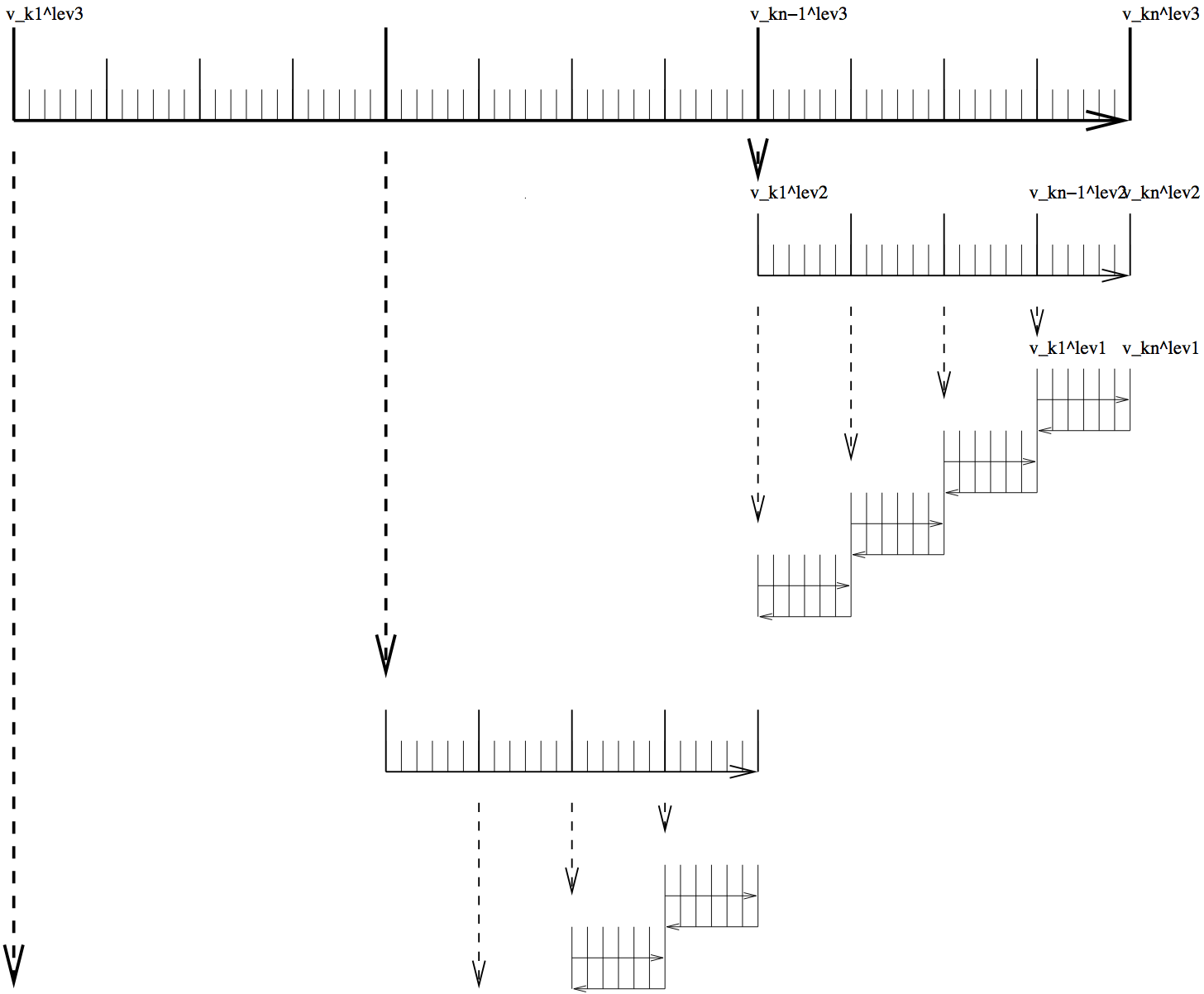
Restrepo et al., 1998 [RLG98]). It is depicted in Figure 7.1 for
a 3-level checkpointing (as an example, we give explicit numbers for a
3-day integration with a 1-hourly timestep in square brackets).
Figure 7.1 Schematic view of intermediate dump and restart for 3-level checkpointing.
In a first step, the model trajectory is subdivided into
\({n}^{lev3}\) subsections [\({n}^{lev3}\)=3 1-day
intervals], with the label \(lev3\) for this outermost loop. The
model is then integrated along the full trajectory, and the model
state stored to disk only at every \(k_{i}^{lev3}\)-th timestep
[i.e. 3 times, at \(i = 0,1,2\) corresponding to
\(k_{i}^{lev3} = 0, 24, 48\)]. In addition, the cost function
is computed, if needed.
In a second step each subsection itself is divided into
\({n}^{lev2}\) subsections [\({n}^{lev2}\)=4 6-hour
intervals per subsection]. The model picks up at the last outermost
dumped state \(v_{k_{n}^{lev3}}\) and is integrated forward in
time along the last subsection, with the label \(lev2\) for this
intermediate loop. The model state is now stored to disk at every
\(k_{i}^{lev2}\)-th timestep [i.e. 4 times, at
\(i = 0,1,2,3\) corresponding to
\(k_{i}^{lev2} = 48, 54, 60, 66\)].
Finally, the model picks up at the last intermediate dump state
\(v_{k_{n}^{lev2}}\) and is integrated forward in time along
the last subsection, with the label \(lev1\) for this
intermediate loop. Within this sub-subsection only, parts of the
model state are stored to memory at every timestep [i.e. every hour
\(i=0,...,5\) corresponding to
\(k_{i}^{lev1} = 66, 67, \ldots, 71\)]. The final state
\(v_n = v_{k_{n}^{lev1}}\) is reached and the model state of
all preceding timesteps along the last innermost subsection are
available, enabling integration backwards in time along the last
subsection. The adjoint can thus be computed along this last
subsection \(k_{n}^{lev2}\).
This procedure is repeated consecutively for each previous subsection
\(k_{n-1}^{lev2}, \ldots, k_{1}^{lev2}\) carrying the adjoint
computation to the initial time of the subsection \(k_{n}^{lev3}\).
Then, the procedure is repeated for the previous subsection
\(k_{n-1}^{lev3}\) carrying the adjoint computation to the initial
time \(k_{1}^{lev3}\).
For the full model trajectory of
\(n^{lev3} \cdot n^{lev2} \cdot n^{lev1}\) timesteps the required
storing of the model state was significantly reduced to
\(n^{lev2} + n^{lev3}\) to disk and roughly \(n^{lev1}\) to
memory (i.e., for the 3-day integration with a total of 72 timesteps the
model state was stored 7 times to disk and roughly 6 times to memory).
This saving in memory comes at a cost of a required 3 full forward
integrations of the model (one for each checkpointing level). The
optimal balance of storage vs. recomputation certainly depends on the
computing resources available and may be adjusted by adjusting the
partitioning among the \(n^{lev3}, \,\, n^{lev2}, \,\, n^{lev1}\).
In this section we describe in a general fashion the parts of the code
that are relevant for automatic differentiation using the software tool
TAF. Modifications to use OpenAD are described in Section 7.5.
If CPP option
ALLOW_AUTODIFF_TAMC is defined, the driver routine
the_model_main.F,
instead of calling the_model_loop.F, invokes the
adjoint of this routine, adthe_main_loop.F (case
#define ALLOW_ADJOINT_RUN, or the tangent linear of this routine
g_the_main_loop.F (case #define ALLOW_TANGENTLINEAR_RUN), which
are the toplevel routines in terms of automatic differentiation. The
routines adthe_main_loop.F or g_the_main_loop.F are generated by
TAF. It contains both the forward integration of the full model, the
cost function calculation, any additional storing that is required for
efficient checkpointing, and the reverse integration of the adjoint
model.
[DESCRIBE IN A SEPARATE SECTION THE WORKING OF THE TLM]
The above structure of adthe_main_loop.F has been
strongly simplified to focus on the essentials; in particular, no
checkpointing procedures are shown here. Prior to the call of
adthe_main_loop.F, the routine ctrl_unpack.F
is invoked to unpack the
control vector or initialize the control variables. Following the call
of adthe_main_loop.F, the routine ctrl_pack.F
is invoked to pack the
control vector (cf. Section 7.2.5). If gradient checks are to
be performed, the option #define ALLOW_GRDCHK is chosen. In this case
the driver routine grdchk_main.F
is called after the gradient has been
computed via the adjoint (cf. Section 7.3).
The build process of an AD code is very similar to building the forward
model. However, depending on which AD code one wishes to generate, and
on which AD tool is available (TAF or TAMC), the following make targets
are available:
AD-target
output
description
«MODE»«TOOL»only
«MODE»_«TOOL»_output.f
generates code for «MODE» using «TOOL»
no make dependencies on .F .h
useful for compiling on remote platforms
«MODE»«TOOL»
«MODE»_«TOOL»_output.f
generates code for «MODE» using «TOOL»
includes make dependencies on .F .h
i.e. input for «TOOL» may be re-generated
«MODE»all
mitgcmuv_«MODE»
generates code for «MODE» using «TOOL»
and compiles all code
(use of TAF is set as default)
Here, the following placeholders are used:
«TOOL»
TAF
TAMC
«MODE»
ad generates the adjoint model (ADM)
ftl generates the tangent linear model (TLM)
svd generates both ADM and TLM for
singular value decomposition (SVD) type calculations
For example, to generate the adjoint model using TAF after routines (.F)
or headers (.h) have been modified, but without compilation,
type makeadtaf; or, to generate the tangent linear model using TAMC without
re-generating the input code, type makeftltamconly.
A typical full build process to generate the ADM via TAF would look like
follows:
% mkdir build
% cd build
% ../../../tools/genmake2 -mods=../code_ad [ -nocat4ad ]
% make depend
% make adall
The make«MODE»all target consists of the following procedures:
A header file AD_CONFIG.h is generated which contains a CPP option
on which code ought to be generated. Depending on the make target,
the contents is one of the following:
If `` -nocat4ad`` is not specified, a single file «MODE»_input_code.f is
concatenated consisting of all .f files that are part of the list
AD_FILES and all .flow files that are part of the list
AD_FLOW_FILES.
The AD tool is invoked with the «MODE»_«TOOL»_FLAGS. The default AD tool
flags in genmake2 can be overwritten by a
tools/adjoint_options file (similar to the platform-specific
tools/build_options, see Section 3.5.2.2). The AD
tool writes the resulting AD code into the file «MODE»_input_code_ad.f.
A short sed script tools/adjoint_sed is
applied to «MODE»_input_code_ad.f to reinstate myThid into
the CALL argument list of active file I/O. The result is written to file
«MODE»_«TOOL»_output.f.
If the `` -nocat4ad`` option is specified, the concatenation of all .f
files is skipped and instead all necessary files are sent to TAF and for
each file an AD-file is returned.
All routines are compiled and an executable is generated.
7.2.3.1. The list AD_FILES and *_ad_diff.list files
Not all routines are presented to the AD tool. Routines typically hidden
are diagnostics routines which do not influence the cost function, but
may create artificial flow dependencies such as I/O of active variables.
genmake2 generates a list (or variable) AD_FILES
that contains all routines that are shown to the AD tool.
This list is put together from all files with suffix _ad_diff.list
that genmake2 finds in its search directories.
The list file for the core MITgcm routines is model/src/model_ad_diff.list.
Note that no wrapper routine is shown to TAF. These are either not visible at
all to the AD code, or hand-written AD code is available (see next section).
Each package directory contains its package-specific list file
«PKG»_ad_diff.list. For example, pkg/ptracers contains the file
ptracers_ad_diff.list.
Thus, enabling a package will automatically
extend the AD_FILES list of genmake2 to incorporate the
package-specific routines. Note that you will need to regenerate the
makefile if you enable a package (e.g., by adding it to packages.conf)
and a Makefile already exists.
TAMC and TAF can evaluate user-specified directives that start with a
specific syntax (CADJ, C$TAF, !$TAF). The main categories of directives
are STORE directives and FLOW directives. Here, we are concerned with
flow directives, store directives are treated elsewhere.
Flow directives enable the AD tool to evaluate how it should treat
routines that are ’hidden’ by the user, i.e. routines which are not
contained in the AD_FILES list (see previous section), but which
are called in part of the code that the AD tool does see. The flow
directive tell the AD tool:
which subroutine arguments are input/output
which subroutine arguments are active
which subroutine arguments are required to compute the cost
which subroutine arguments are dependent
The syntax for the flow directives can be found in the AD tool manuals.
genmake2 generates a list (or variable) AD_FLOW_FILES
that contains all files with suffix .flow that it finds in its search
directories. The flow directives for the core MITgcm routines of
eesupp/src/ and model/src/ reside in pkg/autodiff/. This directory also
contains hand-written adjoint code for the MITgcm WRAPPER (Section 6.2).
Flow directives for package-specific routines are contained in the
corresponding package directories, generally in a file «PKG»_ad.flow, e.g.,
ptracers-specific directives are in ptracers_ad.flow.
7.2.3.3. Store directives for 3-level checkpointing
The storing that is required at each period of the 3-level checkpointing
is controlled by three top-level headers.
do ilev_3 = 1, nchklev_3
#  include ``checkpoint_lev3.h''
   do ilev_2 = 1, nchklev_2
#     include ``checkpoint_lev2.h''
      do ilev_1 = 1, nchklev_1
#        include ``checkpoint_lev1.h''

...

      end do
   end do
end do
All files checkpoint_lev?.h are contained in directory pkg/autodiff/.
7.2.3.4. Changing the default AD tool flags: ad_options files
The cost function \({\cal J}\) is referred to as the dependent
variable. It is a function of the input variables \(\vec{u}\) via
the composition
\({\cal J}(\vec{u}) \, = \, {\cal J}(M(\vec{u}))\). The input are
referred to as the independent variables or control variables. All
aspects relevant to the treatment of the cost function
\({\cal J}\) (parameter setting, initialization, accumulation,
final evaluation), are controlled by the package pkg/cost. The aspects
relevant to the treatment of the independent variables are controlled by
the package pkg/ctrl and will be treated in the next section.
pkg/cost is enabled by adding the line cost to your
file packages.conf (see Section 8.1.1).
In general the following packages ought to be enabled simultaneously:
pkg/autodiff, pkg/ctrl, and
pkg/cost. The basic CPP option to enable the cost function is
ALLOW_COST. Each specific cost function contribution has its own
option. For the present example the option is ALLOW_COST_TRACER. All
cost-specific options are set in COST_OPTIONS.h. Since the cost function is usually used in
conjunction with automatic differentiation, the CPP option
ALLOW_AUTODIFF_TAMC (file AUTODIFF_OPTIONS.h) should be defined.
The initialization of pkg/cost is readily enabled as soon as
the CPP option ALLOW_COST is defined.
The S/R cost_readparms.F
reads runtime flags and parameters from file data.cost.
For the present example the only relevant parameter read is
mult_tracer. This multiplier enables different cost function
contributions to be switched on (=1.) or off (=0.) at runtime.
For more complex cost functions which involve model vs. data
misfits, the corresponding data filenames and data specifications
(start date and time, period, …) are read in this S/R.
The S/R cost_init_varia.F
initializes the different cost function contributions. The
contribution for the present example is objf_tracer which is
defined on each tile (bi,bj).
The ’driver’ routine cost_tile.F
is called at the end of each time
step. Within this ’driver’ routine, S/R are called for each of the
chosen cost function contributions. In the present example
(ALLOW_COST_TRACER), S/R cost_tracer.F is called. It accumulates
objf_tracer according to eqn. (ref:ask-the-author).
At the end of the forward integration S/R cost_final.F is called. It
accumulates the total cost function fc from each contribution and
sums over all tiles:
7.2.5. The control variables (independent variables)
The control variables are a subset of the model input (initial
conditions, boundary conditions, model parameters). Here we identify
them with the variable \(\vec{u}\). All intermediate variables
whose derivative with respect to control variables do not vanish are called
active variables. All subroutines whose derivative with respect to the control
variables don’t vanish are called active routines. Read and write
operations from and to file can be viewed as variable assignments.
Therefore, files to which active variables are written and from which
active variables are read are called active files. All aspects relevant
to the treatment of the control variables (parameter setting,
initialization, perturbation) are controlled by the package pkg/ctrl.
Package pkg/ctrl is enabled by adding the line ctrl to your
file packages.conf. Each control variable is enabled via its own CPP
option in CTRL_OPTIONS.h.
The S/R ctrl_readparms.F
reads runtime flags and parameters from file data.ctrl.
For the present example the file contains the file names of each
control variable that is used. In addition, the number of wet
points for each control variable and the net dimension of the space
of control variables (counting wet points only) nvarlength is
determined. Masks for wet points for each tile (bi,bj) and
vertical layer k are generated for the three relevant
categories on the C-grid: nWetCtile for tracer fields,
nWetWtile for zonal velocity fields, nWetStile for
meridional velocity fields.
Two important issues related to the handling of the control
variables in MITgcm need to be addressed. First, in order to save
memory, the control variable arrays are not kept in memory, but
rather read from file and added to the initial fields during the
model initialization phase. Similarly, the corresponding adjoint
fields which represent the gradient of the cost function with respect to the
control variables are written to file at the end of the adjoint
integration. Second, in addition to the files holding the 2-D
and 3-D control variables and the corresponding cost gradients,
a 1-D control vector and gradient vector are written to file.
They contain only the wet points of the control variables and the
corresponding gradient. This leads to a significant data
compression. Furthermore, an option is available
(ALLOW_NONDIMENSIONAL_CONTROL_IO) to non-dimensionalize the
control and gradient vector, which otherwise would contain
different pieces of different magnitudes and units. Finally, the
control and gradient vector can be passed to a minimization routine
if an update of the control variables is sought as part of a
minimization exercise.
The files holding fields and vectors of the control variables and
gradient are generated and initialized in S/R ctrl_unpack.F.
7.2.5.3. Perturbation of the independent variables
The dependency flow for differentiation with respect to the controls starts with
adding a perturbation onto the input variable, thus defining the
independent or control variables for TAF. Three types of controls may be
considered:
Consider as an example the initial tracer distribution pTracer as
control variable. After pTracer has been initialized in
ptracers_init_varia.F
(dynamical variables such as temperature and salinity are
initialized in ini_fields.F), a perturbation anomaly is added to
the field in S/R ctrl_map_ini.F:
xx_tr1 is a 3-D global array holding the perturbation. In
the case of a simple sensitivity study this array is identical to
zero. However, it’s specification is essential in the context of
automatic differentiation since TAF treats the corresponding line
in the code symbolically when determining the differentiation chain
and its origin. Thus, the variable names are part of the argument
list when calling TAF:
taf -input 'xx_tr1 ...' ...
Now, as mentioned above, MITgcm avoids maintaining an array for each
control variable by reading the perturbation to a temporary array
from file. To ensure the symbolic link to be recognized by TAF, a
scalar dummy variable xx_tr1_dummy is introduced and an ’active
read’ routine of the adjoint support package pkg/autodiff is
invoked. The read-procedure is tagged with the variable
xx_tr1_dummy enabling TAF to recognize the initialization of
the perturbation. The modified call of TAF thus reads
taf -input 'xx_tr1_dummy ...' ...
and the modified operation (to perturb) in the code takes on the
form
Note that reading an active variable corresponds to a variable
assignment. Its derivative corresponds to a write statement of the
adjoint variable, followed by a reset. The ’active file’ routines
have been designed to support active read and corresponding adjoint
active write operations (and vice versa).
The handling of boundary values as control variables proceeds
exactly analogous to the initial values with the symbolic
perturbation taking place in S/R
ctrl_map_forcing.F.
Note however
an important difference: Since the boundary values are time
dependent with a new forcing field applied at each time step, the
general problem may be thought of as a new control variable at each
time step (or, if the perturbation is averaged over a certain
period, at each \(N\) timesteps), i.e.,
In the current example an equilibrium state is considered, and
only an initial perturbation to surface forcing is applied with
respect to the equilibrium state. A time dependent treatment of the
surface forcing is implemented in the ECCO environment, involving
the calendar (pkg/cal) and external forcing (pkg/exf) packages.
This routine is not yet implemented, but would proceed proceed
along the same lines as the initial value sensitivity. The mixing
parameters diffkr and kapgm are currently added as controls
in ctrl_map_ini.F.
7.2.5.4. Output of adjoint variables and gradient
Several ways exist to generate output of adjoint fields.
The control variable fields xx\_«...»: before the forward integration, the control variables are read
from file «xx\_...» and added to the model field.
The adjoint variable fields adxx\_«...», i.e., the gradient
\(\nabla _{u}{\cal J}\) for each control variable:
after the adjoint integration the corresponding adjoint
variables are written to adxx\_«...».
The control vector vector_ctrl:
at the very beginning of the model initialization, the updated
compressed control vector is read (or initialized) and
distributed to 2-D and 3-D control variable fields.
The gradient vector vector_grad:
at the very end of the adjoint integration, the 2-D and
3-D adjoint variables are read, compressed to a single vector
and written to file.
In addition to writing the gradient at the end of the
forward/adjoint integration, many more adjoint variables of the
model state at intermediate times can be written using S/R
addummy_in_stepping.F.
The procedure is
enabled using via the CPP-option ALLOW_AUTODIFF_MONITOR (file
AUTODIFF_OPTIONS.h).
To be part of the adjoint code, the
corresponding S/R dummy_in_stepping.F
has to be called in the
forward model (S/R the_main_loop.F) at the appropriate place. The
adjoint common blocks are extracted from the adjoint code via the
header file adcommon.h.
dummy_in_stepping.F is essentially empty, the corresponding adjoint
routine is hand-written rather than generated automatically.
Appropriate flow directives
(dummy_in_stepping.flow)
ensure that
TAMC does not automatically generate addummy_in_stepping.F by
trying to differentiate dummy_in_stepping.F, but instead refers to
the hand-written routine.
WARNING: If the structure of the common blocks dynvars_r,
dynvars_cd, etc., changes similar changes will occur in the
adjoint common blocks. Therefore, consistency between the
TAMC-generated common blocks and those in
adcommon.h have to be
checked.
7.2.5.5. Control variable handling for optimization applications
In optimization mode the cost function \({\cal J}(u)\) is sought
to be minimized with respect to a set of control variables
\(\delta {\cal J} \, = \, 0\), in an iterative manner. The
gradient \(\nabla _{u}{\cal J} |_{u_{[k]}}\) together with the
value of the cost function itself \({\cal J}(u_{[k]})\) at
iteration step \(k\) serve as input to a minimization routine
(e.g. quasi-Newton method, conjugate gradient, … (Gilbert and Lemaréchal, 1989
[GLemarechal89]) to compute an update in the control
variable for iteration step \(k+1\):
\(u_{[k+1]}\) then serves as input for a forward/adjoint run to
determine \({\cal J}\) and \(\nabla _{u}{\cal J}\) at
iteration step \(k+1\). Figure 7.2 sketches the flow
between forward/adjoint model and the minimization routine.
Figure 7.2 Flow between the forward/adjoint model and the minimization routine.
The routines ctrl_unpack.F and
ctrl_pack.F provide the link between
the model and the minimization routine. As described in Section
ref:ask-the-author the ctrl_unpack.F
and ctrl_pack.F routines read and write
control and gradient vectors which are compressed to contain only wet
points, in addition to the full 2-D and 3-D fields. The
corresponding I/O flow is shown in Figure 7.3:
Figure 7.3 Flow chart showing I/O in the forward/adjoint model.
ctrl_unpack.F reads the updated control
vector vector_ctrl_<k>. It distributes the different control variables to
2-D and 3-D files xx_«...»<k>. At the start of the forward integration the
control variables are read from xx_«...»<k> and added to the field.
Correspondingly, at the end of the adjoint integration the adjoint fields are
written to adxx_«...»<k>, again via the active file routines. Finally,
ctrl_pack.F collects all adjoint files and
writes them to the compressed vector file vector_grad_<k>.
An indispensable test to validate the gradient computed via the adjoint
is a comparison against finite difference gradients. The gradient check
package pkg/grdchk enables such tests in a straightforward and easy
manner. The driver routine grdchk_main.F is called from
the_model_main.F after
the gradient has been computed via the adjoint
model (cf. flow chart ???).
The gradient check proceeds as follows: The \(i-\)th component of
the gradient \((\nabla _{u}{\cal J}^T)_i\) is compared with the
following finite-difference gradient:
A gradient check at point \(u_i\) may generally considered to be
successful if the deviation of the ratio between the adjoint and the
finite difference gradient from unity is less than 1 percent,
the_model_main
|
|-- ctrl_unpack
|-- adthe_main_loop            - unperturbed cost function and
|-- ctrl_pack                    adjoint gradient are computed here
|
|-- grdchk_main
    |
    |-- grdchk_init
    |-- do icomp=...           - loop over control vector elements
        |
        |-- grdchk_loc         - determine location of icomp on grid
        |
        |-- grdchk_getxx       - get control vector component from file
        |                        perturb it and write back to file
        |-- grdchk_getadxx     - get gradient component calculated
        |                        via adjoint
        |-- the_main_loop      - forward run and cost evaluation
        |                        with perturbed control vector element
        |-- calculate ratio of adj. vs. finite difference gradient
        |
        |-- grdchk_setxx       - Reset control vector element
        |
        |-- grdchk_print       - print results
Authors: Patrick Heimbach & Geoffrey Gebbie, 07-Mar-2003
*NOTE:THIS SECTION IS SUBJECT TO CHANGE. IT REFERS TO TAF-1.4.26.
Old TAF versions are incomplete and have problems with both TAF options
-pure and -mpi. At the time of the latest update, the current version
of TAF is 6.1.5
Most high performance computing (HPC) centers require the use of batch
jobs for code execution. Limits in maximum available CPU time and memory
may prevent the adjoint code execution from fitting into any of the
available queues. This presents a serious limit for large scale / long
time adjoint ocean and climate model integrations. The MITgcm itself
enables the split of the total model integration into sub-intervals
through standard dump/restart of/from the full model state. For a
similar procedure to run in reverse mode, the adjoint model requires, in
addition to the model state, the adjoint model state, i.e., all variables
with derivative information which are needed in an adjoint restart. This
adjoint dump & restart is also termed ’divided adjoint (DIVA)’.
For this to work in conjunction with automatic differentiation, an AD
tool needs to perform the following tasks:
identify an adjoint state, i.e., those sensitivities whose
accumulation is interrupted by a dump/restart and which influence the
outcome of the gradient. Ideally, this state consists of
the adjoint of the model state,
the adjoint of other intermediate results (such as control
variables, cost function contributions, etc.)
bookkeeping indices (such as loop indices, etc.)
generate code for storing and reading adjoint state variables
generate code for bookkeeping , i.e., maintaining a file with index
information
generate a suitable adjoint loop to propagate adjoint values for
dump/restart with a minimum overhead of adjoint intermediate values.
TAF (but not TAMC!) generates adjoint code which performs the above
specified tasks. It is closely tied to the adjoint multi-level
checkpointing. The adjoint state is dumped (and restarted) at each step
of the outermost checkpointing level and adjoint integration is
performed over one outermost checkpointing interval. Prior to the
adjoint computations, a full forward sweep is performed to generate the
outermost (forward state) tapes and to calculate the cost function. In
the current implementation, the forward sweep is immediately followed by
the first adjoint leg. Thus, in theory, the following steps are
performed (automatically)
1st model call:
This is the case if file costfinal does not exist. S/R
mdthe_main_loop.f (generated by TAF) is called.
calculate forward trajectory and dump model state after each
outermost checkpointing interval to files tapelev3
calculate cost function fc and write it to file costfinal
2nd and all remaining model calls:
This is the case if file costfinal does exist. S/R
adthe_main_loop.f (generated by TAF) is called.
(forward run and cost function call is avoided since all values
are known)
if 1st adjoint leg:
create index file divided.ctrl which contains info on current
checkpointing index \(ilev3\)
if not \(i\)-th adjoint leg:
adjoint picks up at \(ilev3 = nlev3-i+1\) and runs to
\(nlev3 - i\)
perform adjoint leg from \(nlev3-i+1\) to \(nlev3 - i\)
dump adjoint state to file snapshot
dump index file divided.ctrl for next adjoint leg
in the last step the gradient is written.
A few modifications were performed in the forward code, obvious ones
such as adding the corresponding TAF-directive at the appropriate place,
and less obvious ones (avoid some re-initializations, when in an
intermediate adjoint integration interval).
[For TAF-1.4.20 a number of hand-modifications were necessary to
compensate for TAF bugs. Since we refer to TAF-1.4.26 onwards, these
modifications are not documented here].
7.4.2. Recipe for divided adjoint code generation
Verification experiment lab_sea tests the
divided adjoint and serves as an example of how to configure the code.
define USE_DIVA=1, either as an environment variable (e.g., in bash:
exportUSE_DIVA=1), in a genmake_local file in the build
directory, or in your build options file. This will instruct
genmake2 to generate TAF options (-pure)
for divided adjoint generation.
If using MPI, make sure that the paths to mpi-header files, such as
mpif.h, are know to genmake2 (as usual, via
the build options file, see also Section 7.4.3).
Run the usual sequence for generating the Makefile and the AD-code.
../../../tools/genmake2  -mods=../code_ad -nocat4ad [ other options ]
make depend
make adtaf
the -nocat4ad option is not necessary, but will generate individual
AD-files for each forward file sent to TAF. The adjoint code now contains
subroutines (in the_main_loop_ad.f):
adthe_main_loop_ad:
Is responsible for the forward trajectory, storing of outermost
checkpoint levels to file, computation of cost function, and
storing of cost function to file (1st step).
adthe_main_loop:
Is responsible for computing one adjoint leg, dump adjoint state
to file and write index info to file (2nd and consecutive
steps).
Then compile with makeadall (the makeadtaf step is not necessary
unless you want to inspect the TAF-generated code before compiling).
7.4.3. Special considerations for multi processor (MPI) runs
On the machine where you execute the code (most likely not the machine where
you run TAF) find the includes directory for MPI containing mpif.h. Either
copy mpif.h to the machine where you preprocess the code (generate the
.f files) before TAF-ing, or add the path to the includes directory to your
genmake2 platform setup. TAF needs some MPI
parameter settings (essentially mpi_comm_world and mpi_integer) to
incorporate those in the adjoint code. The -mpi will be added to the TAF
argument list automatically.
IMPORTANT NOTE: As OpenAD is no longer maintained (latest OpenAD snapshot
at Argonne National Lab was from March 2014), MITgcm stopped supporting the
OpenAD interface after the checkpoint69o tag (from July 2026). In case you
need to use OpenAD for a specific application, please use the last OpenAD
supported code:
% git checkout checkpoint69o
Authors: Jean Utke, Patrick Heimbach and Chris Hill
The development of OpenAD was initiated as part of the ACTS (Adjoint
Compiler Technology & Standards) project funded by the NSF Information
Technology Research (ITR) program. The main goals for OpenAD initially
defined for the ACTS project are:
develop a flexible, modular, open source tool that can generate
adjoint codes of numerical simulation programs,
establish a platform for easy implementation and testing of source
transformation algorithms via a language-independent abstract
intermediate representation,
support for source code written in C and Fortan, and
generate efficient tangent linear and adjoint for the MIT general
circulation model.
The OpenAD webpage has a detailed description on how to download and
build OpenAD. From its homepage, please click on
Binaries. You may either download pre-built binaries
for quick trial, or follow the detailed build process described at
http://www.mcs.anl.gov/OpenAD/access.shtml.
7.5.4. Building the MITgcm adjoint using an OpenAD Singularity container
The MITgcm adjoint can also be built using a Singularity container. You will
need Singularity, version 3.X. A container
with OpenAD can be downloaded from the Sylabs Cloud: 1
The -oadsingularity option is also supported by testreport,
Section 5.5.2. Note that the path to the container has to be
either absolute or relative to the build directory.
Please refer to Gaikwad et al. (2024) [GNH+25] for more details and a comparative analysis with TAF. Recently, introduction of the profiling capabilities in Tapenade have resulted in substantial insights and speedups for the Tapenade-generated adjoint, see Hascoet et al. (2024) [HBG+24].
Feel free to reach out if you wish to use Tapenade and need help!
Authors: Shreyas Sunil Gaikwad, Sri Hari Krishna Naryanan, Laurent Hascoet, Patrick
Heimbach
TAPENADE is an open-source Automatic Differentiation Engine developed at INRIA
Sophia-Antipolis by the Tropics then Ecuador teams. TAPENADE can be utilized as
a server (JAVA servlet), which runs at INRIA Sophia-Antipolis. The current
address of this TAPENADE server is here. TAPENADE can also be
downloaded and installed locally as a set of JAVA classes (JAR archive). In
that case it is run by a simple command line, which can be included into a
Makefile. It also provides you with a user-interface to visualize the results
in a HTML browser.
While the MITgcm source files are prepared to generate adjoint sensitivities,
they will not be able to do so without an operable installation of
Tapenade. Fortunately the Tapenade installation procedure is straight forward.
We detail the instructions here, but the latest instructions can always be
found here.
Before installing Tapenade, you must check that an up-to-date Java Runtime
Environment is installed. Tapenade will not run with older Java Runtime
Environment.
Tapenade 3.16 distribution does not contain a fortranParser executable
for MacOS. You need docker on your Mac to run the Tapenade
distribution with Fortran programs with a docker image from here. Details on how to
build your own fortranParser is here.
You may also build Tapenade on your Mac from the gitlab repository.
use the option -rootdir at the genmake2 step, or alternatively export environment
variable MITGCM_ROOTDIR, to specify the absolute path to your
MITgcm directory (see also Section 3.5.2.1).
bind mount the absolute path in the docker command as a volume by putting
in your build-options or in a genmake_local file
(Section 3.5.2). BASENAME should expand to your
root directory (check TAPENADECMD in Makefile).
In order to run ./testreport -tap $moreoption in verification,
the root directory can be passed to genmake2 via exportMITGCM_ROOTDIR=$BASEDIR or setting it
in your built-options or genmake_local file.
Download tapenade_3.16.tar
into your chosen installation directory install_dir.
Go to your chosen installation directory install_dir, and extract Tapenade
from the tar file :
% tar xvfz tapenade_3.16.tar
On Linux, depending on your distribution, Tapenade may require you to set
the shell variable JAVA_HOME to your java installation directory. It is
often JAVA_HOME=/usr/java/default. You might also need to modify the
PATH by adding the bin directory from the Tapenade installation. An
example can be found here.
Before installing Tapenade, you must check that an up-to-date Java Runtime
Environment is installed. Tapenade will not run with older Java Runtime
Environment. The Fortran parser of Tapenade uses cygwin.
Download tapenade_3.16.zip
into your chosen installation directory install_dir.
Go to your chosen installation directory install_dir, and extract Tapenade
from the zip file.
Save a copy of the install_dir\tapenade_3.16\bin\tapenade.bat file and
modify install_dir\tapenade_3.16\bin\tapenade.bat according to your
installation parameters:
replace TAPENADE_HOME=.. by TAPENADE_HOME="install_dir"\tapenade_3.16
replace JAVA_HOME="C:\Progra~1\Java\jdkXXXX" by your current java directory
replace BROWSER="C:\ProgramFiles\InternetExplorer\iexplore.exe" by your
current browser.
NOTE: Every time you wish to use the AD capability with Tapenade, you must re-source the environment. We recommend that this be done automatically in your bash or c-shell profile upon login. An example of an addition to a .bashrc file from a Linux server is given below. Luckily, shell variable JAVA_HOME was not required to be explicitly set for this particular Linux distribution, but might be necessary for some other distributions.
##set some env variables for tapenade

export TAPENADE_HOME="/home/shreyas/tapenade_3.16"
export PATH="$PATH:$TAPENADE_HOME/bin"

##Modules

module use /share/modulefiles/
module load java/jdk/16.0.1 # Java required by Tapenade
You should now have a working copy of Tapenade.
For more information on the tapenade command and its arguments, type :
The packages.conf file should include both the adjoint and tapenade
packages. Note that mnc and ecco packages are not yet compatible with
Tapenade. The users are referred to the code_tap directories in the various
verification experiments for reference.
Pro tip: diff-qrdir1dir2 can help you see all the differences in the files of two directories.
autodiff is not completely untangled from the Tapenade setup yet. In
code_tap/AUTODIFF_OPTIONS.h, the only flag that can be defined safely is
ALLOW_AUTODIFF_MONITOR.
The setup remains similar to how one sets up the TLM with TAF. A typical flow
will look as follows -
### Assuming $PWD is the build subdirectory
### Clean stuff
make CLEAN

### Use your own optfile
../../../tools/genmake2 -tap -of ../../../tools/build_options/linux_amd64_ifort -mods ../code_tap
make depend

### Differentiate code to generate TLM code using Tapenade
### Creates executable mitgcmuv_tap_tlm
make -j 8 tap_tlm

### Rest of the setup is standard
cd ../run
rm -r *
ln -s ../input_tap/* .
./prepare_run
ln -s ../build/mitgcmuv_tap_tlm .
./mitgcmuv_tap_tlm > output_tap_tlm.txt 2>&1
The setup remains similar to how one sets up the adjoint with TAF. A typical
flow will look as follows -
### Assuming $PWD is the build subdirectory
### Clean stuff
make CLEAN

### Use your own optfile
../../../tools/genmake2 -tap -of ../../../tools/build_options/linux_amd64_ifort -mods ../code_tap
make depend

### Differentiate code to generate adjoint code using Tapenade
### Creates executable mitgcmuv_tap_adj
make -j 8 tap_adj

### Rest of the setup is standard
### These commands are for a typical verification experiment
cd ../run
rm -r *
ln -s ../input_tap/* .
./prepare_run
ln -s ../build/mitgcmuv_tap_adj .
./mitgcmuv_tap_adj > output_tap_adj.txt 2>&1