This chapter focuses on describing the WRAPPER environment within
which both the core numerics and the pluggable packages operate. The
description presented here is intended to be a detailed exposition and
contains significant background material, as well as advanced details on
working with the WRAPPER. The tutorial examples in this manual (see
Section 4) contain more
succinct, step-by-step instructions on running basic numerical
experiments, of various types, both sequentially and in parallel. For
many projects, simply starting from an example code and adapting it to
suit a particular situation will be all that is required. The first part
of this chapter discusses the MITgcm architecture at an abstract level.
In the second part of the chapter we described practical details of the
MITgcm implementation and the current tools and operating system features
that are employed.
Broadly, the goals of the software architecture employed in MITgcm are
three-fold:
To be able to study a very broad range of interesting and
challenging rotating fluids problems;
The model code should be readily targeted to a wide range of
platforms; and
On any given platform, performance should be
comparable to an implementation developed and specialized
specifically for that platform.
These points are summarized in Figure 6.1,
which conveys the goals of the MITgcm design. The goals lead to a
software architecture which at the broadest level can be viewed as
consisting of:
A core set of numerical and support code. This is discussed in detail
in Section 2.
A scheme for supporting optional “pluggable” packages (containing
for example mixed-layer schemes, biogeochemical schemes, atmospheric
physics). These packages are used both to overlay alternate dynamics
and to introduce specialized physical content onto the core numerical
code. An overview of the package scheme is given at the start of
Section 8.
A support framework called WRAPPER (Wrappable Application
Parallel Programming Environment Resource), within which the core
numerics and pluggable packages operate.
Figure 6.1 The MITgcm architecture is designed to allow simulation of a wide range of physical problems on a wide range of hardware. The computational resource requirements of the applications targeted range from around 107 bytes ( \(\approx\) 10 megabytes) of memory to 1011 bytes ( \(\approx\) 100 gigabytes). Arithmetic operation counts for the applications of interest range from 109 floating point operations to more than 1017 floating point operations.
This chapter focuses on describing the WRAPPER environment under
which both the core numerics and the pluggable packages function. The
description presented here is intended to be a detailed exposition and
contains significant background material, as well as advanced details on
working with the WRAPPER. The “Getting Started” chapter of this manual
(Section 3) contains more succinct, step-by-step
instructions on running basic numerical experiments both sequentially
and in parallel. For many projects simply starting from an example code
and adapting it to suit a particular situation will be all that is
required.
A significant element of the software architecture utilized in MITgcm is
a software superstructure and substructure collectively called the
WRAPPER (Wrappable Application Parallel Programming Environment
Resource). All numerical and support code in MITgcm is written to “fit”
within the WRAPPER infrastructure. Writing code to fit within the
WRAPPER means that coding has to follow certain, relatively
straightforward, rules and conventions (these are discussed further in
Section 6.3.1).
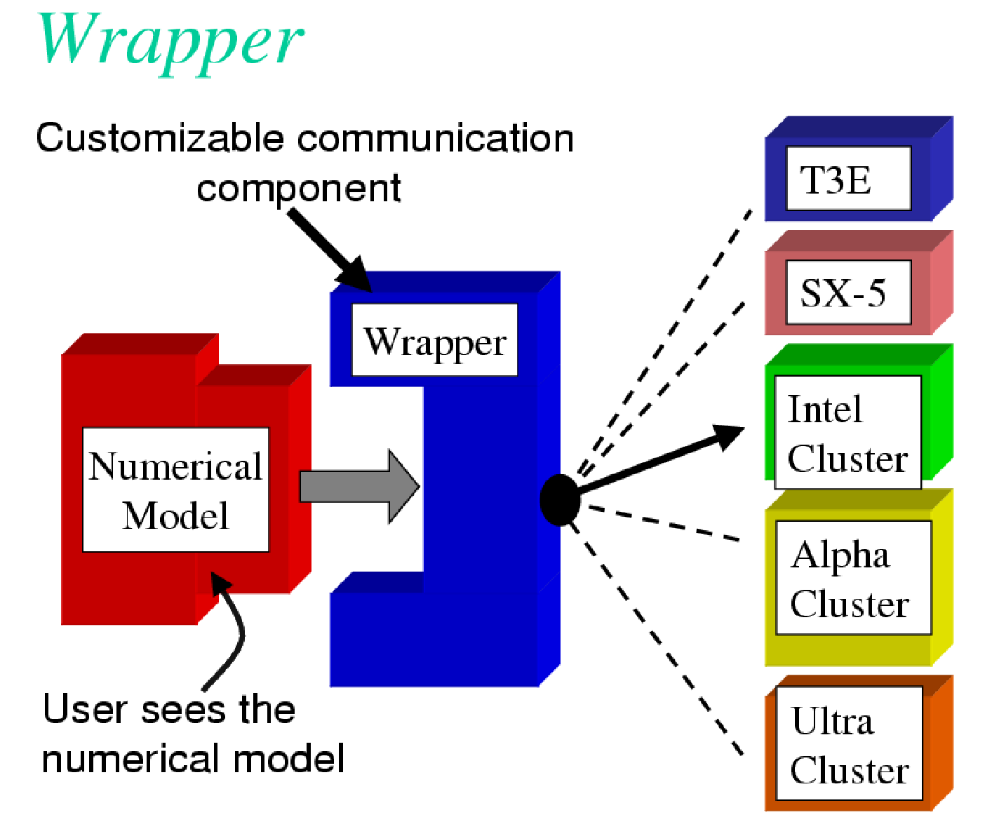
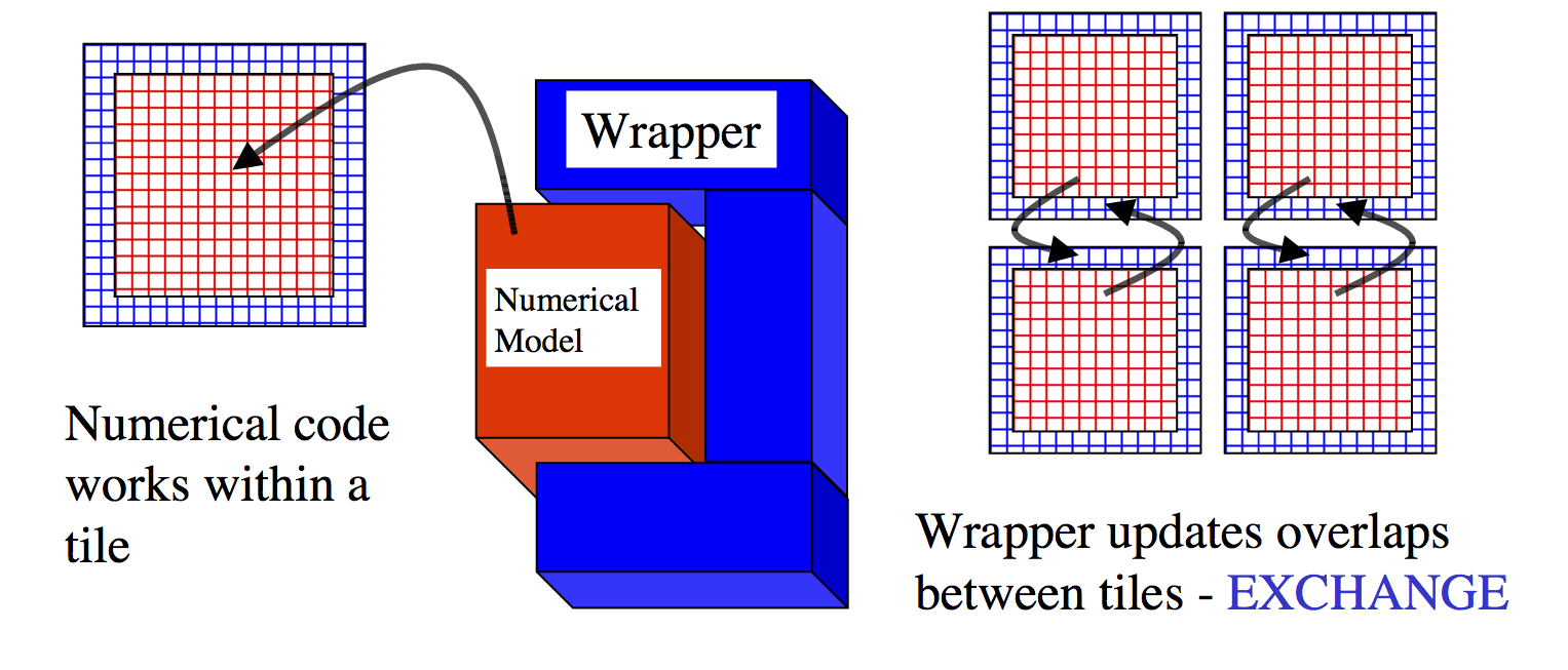
The approach taken by the WRAPPER is illustrated in Figure 6.2,
which shows how the WRAPPER serves to insulate
code that fits within it from architectural differences between hardware
platforms and operating systems. This allows numerical code to be easily
retargeted.
Figure 6.2 Numerical code is written to fit within a software support infrastructure called WRAPPER. The WRAPPER is portable and can be specialized for a wide range of specific target hardware and programming environments, without impacting numerical code that fits within the WRAPPER. Codes that fit within the WRAPPER can generally be made to run as fast on a particular platform as codes specially optimized for that platform.
The WRAPPER is designed to target as broad as possible a range of
computer systems. The original development of the WRAPPER took place on
a multi-processor, CRAY Y-MP system. On that system, numerical code
performance and scaling under the WRAPPER was in excess of that of an
implementation that was tightly bound to the CRAY system’s proprietary
multi-tasking and micro-tasking approach. Later developments have been
carried out on uniprocessor and multiprocessor Sun systems with both
uniform memory access (UMA) and non-uniform memory access (NUMA)
designs. Significant work has also been undertaken on x86 cluster
systems, Alpha processor based clustered SMP systems, and on
cache-coherent NUMA (CC-NUMA) systems such as Silicon Graphics Altix
systems. The MITgcm code, operating within the WRAPPER, is also
routinely used on large scale MPP systems (for example, Cray T3E and IBM
SP systems). In all cases, numerical code, operating within the WRAPPER,
performs and scales very competitively with equivalent numerical code
that has been modified to contain native optimizations for a particular
system (see Hoe et al. 1999) [HHA99] .
The different systems mentioned in Section 6.2.1 can be
categorized in many different ways. For example, one common distinction
is between shared-memory parallel systems (SMP and PVP) and distributed
memory parallel systems (for example x86 clusters and large MPP
systems). This is one example of a difference between compute platforms
that can impact an application. Another common distinction is between
vector processing systems with highly specialized CPUs and memory
subsystems and commodity microprocessor based systems. There are
numerous other differences, especially in relation to how parallel
execution is supported. To capture the essential differences between
different platforms the WRAPPER uses a machine model.
Applications using the WRAPPER are not written to target just one
particular machine (for example an IBM SP2) or just one particular
family or class of machines (for example Parallel Vector Processor
Systems). Instead the WRAPPER provides applications with an abstract
machine model. The machine model is very general; however, it can
easily be specialized to fit, in a computationally efficient manner, any
computer architecture currently available to the scientific computing
community.
Codes operating under the WRAPPER target an abstract machine that is
assumed to consist of one or more logical processors that can compute
concurrently. Computational work is divided among the logical processors
by allocating “ownership” to each processor of a certain set (or sets)
of calculations. Each set of calculations owned by a particular
processor is associated with a specific region of the physical space
that is being simulated, and only one processor will be associated with each
such region (domain decomposition).
In a strict sense the logical processors over which work is divided do
not need to correspond to physical processors. It is perfectly possible
to execute a configuration decomposed for multiple logical processors on
a single physical processor. This helps ensure that numerical code that
is written to fit within the WRAPPER will parallelize with no additional
effort. It is also useful for debugging purposes. Generally, however,
the computational domain will be subdivided over multiple logical
processors in order to then bind those logical processors to physical
processor resources that can compute in parallel.
Computationally, the data structures (e.g., arrays, scalar variables,
etc.) that hold the simulated state are associated with each region of
physical space and are allocated to a particular logical processor. We
refer to these data structures as being owned by the processor to
which their associated region of physical space has been allocated.
Individual regions that are allocated to processors are called
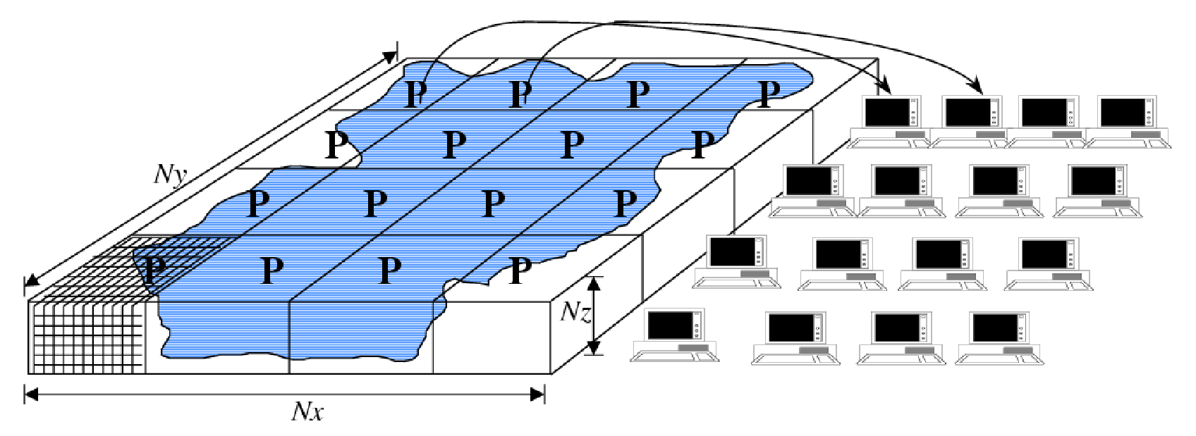
tiles. A processor can own more than one tile. Figure 6.3
shows a physical domain being mapped to a set of
logical processors, with each processor owning a single region of the
domain (a single tile). Except for periods of communication and
coordination, each processor computes autonomously, working only with
data from the tile that the processor owns. If instead multiple
tiles were allotted to a single processor, each of these tiles would be computed on
independently of the other allotted tiles, in a sequential fashion.
Figure 6.3 The WRAPPER provides support for one and two dimensional decompositions of grid-point domains. The figure shows a hypothetical domain of total size \(N_{x}N_{y}N_{z}\). This hypothetical domain is decomposed in two-dimensions along the \(N_{x}\) and \(N_{y}\) directions. The resulting tiles are owned by different processors. The owning processors perform the arithmetic operations associated with a tile. Although not illustrated here, a single processor can own several tiles. Whenever a processor wishes to transfer data between tiles or communicate with other processors it calls a WRAPPER supplied function.
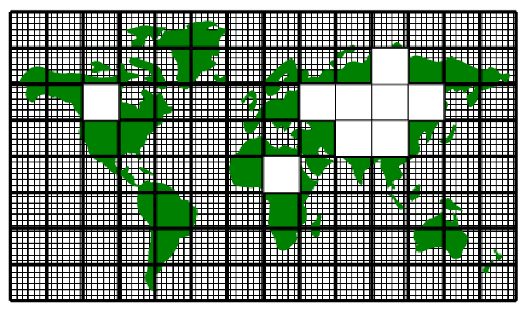
Tiles consist of an interior region and an overlap region. The overlap
region of a tile corresponds to the interior region of an adjacent tile.
In Figure 6.4 each tile would own the region within the
black square and hold duplicate information for overlap regions
extending into the tiles to the north, south, east and west. During
computational phases a processor will reference data in an overlap
region whenever it requires values that lie outside the domain it owns.
Periodically processors will make calls to WRAPPER functions to
communicate data between tiles, in order to keep the overlap regions up
to date (see Section 6.2.6). The WRAPPER
functions can use a variety of different mechanisms to communicate data
between tiles.
Figure 6.4 A global grid subdivided into tiles. Tiles contain a interior region and an overlap region. Overlap regions are periodically updated from neighboring tiles.
Logical processors are assumed to be able to exchange information
between tiles (and between each other) using at least one of two possible
mechanisms, shared memory or distributed memory communication.
The WRAPPER assumes that communication will use one of these two styles.
The underlying hardware and operating system support
for the style used is not specified and can vary from system to system.
Under this mode of communication, data transfers are assumed to be possible using direct addressing of
regions of memory. In the WRAPPER shared memory communication model,
simple writes to an array can be made to be visible to other CPUs at
the application code level. So, as shown below, if one CPU (CPU1) writes
the value 8 to element 3 of array a, then other CPUs (here, CPU2) will be
able to see the value 8 when they read from a(3). This provides a very low
latency and high bandwidth communication mechanism. Thus, in this way one CPU
can communicate information to another CPU by assigning a particular value to a particular memory
location.
  CPU1                    |        CPU2
  ====                    |        ====
                          |
a(3) = 8                  |        WHILE ( a(3) .NE. 8 )
                          |         WAIT
                          |        END WHILE
                          |
Under shared communication independent CPUs are operating on the exact
same global address space at the application level. This is the model of
memory access that is supported at the basic system design level in
“shared-memory” systems such as PVP systems, SMP systems, and on
distributed shared memory systems (e.g., SGI Origin, SGI Altix, and some
AMD Opteron systems). On such systems the WRAPPER will generally use
simple read and write statements to access directly application data
structures when communicating between CPUs.
In a system where assignments statements map directly to hardware instructions that
transport data between CPU and memory banks, this can be a very
efficient mechanism for communication. In such case multiple CPUs
can communicate simply be reading and writing to agreed
locations and following a few basic rules. The latency of this sort of
communication is generally not that much higher than the hardware
latency of other memory accesses on the system. The bandwidth available
between CPUs communicating in this way can be close to the bandwidth of
the systems main-memory interconnect. This can make this method of
communication very efficient provided it is used appropriately.
When using shared memory communication between multiple processors, the
WRAPPER level shields user applications from certain counter-intuitive
system behaviors. In particular, one issue the WRAPPER layer must deal
with is a systems memory model. In general the order of reads and writes
expressed by the textual order of an application code may not be the
ordering of instructions executed by the processor performing the
application. The processor performing the application instructions will
always operate so that, for the application instructions the processor
is executing, any reordering is not apparent. However,
machines are often designed so that reordering of instructions is not
hidden from other second processors. This means that, in general, even
on a shared memory system two processors can observe inconsistent memory
values.
The issue of memory consistency between multiple processors is discussed
at length in many computer science papers. From a practical point of
view, in order to deal with this issue, shared memory machines all
provide some mechanism to enforce memory consistency when it is needed.
The exact mechanism employed will vary between systems. For
communication using shared memory, the WRAPPER provides a place to
invoke the appropriate mechanism to ensure memory consistency for a
particular platform.
Shared-memory machines often have local-to-processor memory caches which
contain mirrored copies of main memory. Automatic cache-coherence
protocols are used to maintain consistency between caches on different
processors. These cache-coherence protocols typically enforce
consistency between regions of memory with large granularity (typically
128 or 256 byte chunks). The coherency protocols employed can be
expensive relative to other memory accesses and so care is taken in the
WRAPPER (by padding synchronization structures appropriately) to avoid
unnecessary coherence traffic.
6.2.5.1.3. Operating system support for shared memory
Applications running under multiple threads within a single process can
use shared memory communication. In this case all the memory locations
in an application are potentially visible to all the compute threads.
Multiple threads operating within a single process is the standard
mechanism for supporting shared memory that the WRAPPER utilizes.
Configuring and launching code to run in multi-threaded mode on specific
platforms is discussed in Section 6.3.2.1.
However, on many systems, potentially very efficient mechanisms for
using shared memory communication between multiple processes (in
contrast to multiple threads within a single process) also exist. In
most cases this works by making a limited region of memory shared
between processes. The MMAP and IPC facilities in UNIX systems provide
this capability as do vendor specific tools like LAPI and IMC.
Extensions exist for the WRAPPER that allow these mechanisms to be used
for shared memory communication. However, these mechanisms are not
distributed with the default WRAPPER sources, because of their
proprietary nature.
Under this mode of communication there is no mechanism, at the application code level,
for directly addressing regions of memory owned and visible to
another CPU. Instead a communication library must be used, as
illustrated below. If one CPU (here, CPU1) writes the value 8 to element 3 of array a,
then at least one of CPU1 and/or CPU2 will need to call a
function in the API of the communication library to communicate data
from a tile that it owns to a tile that another CPU owns. By default
the WRAPPER binds to the MPI communication library
for this style of communication (see https://computing.llnl.gov/tutorials/mpi/
for more information about the MPI Standard).
Many parallel systems are not constructed in a way where it is possible
or practical for an application to use shared memory for communication.
For cluster systems consisting of individual computers connected by
a fast network, there is no notion of shared memory at
the system level. For this sort of system the WRAPPER provides support
for communication based on a bespoke communication library.
The default communication library used is MPI. It is relatively
straightforward to implement bindings to optimized platform specific
communication libraries. For example the work described in
Hoe et al. (1999) [HHA99] substituted standard MPI communication
for a highly optimized library.
Optimized communication support is assumed to be potentially available
for a small number of communication operations. It is also assumed that
communication performance optimizations can be achieved by optimizing a
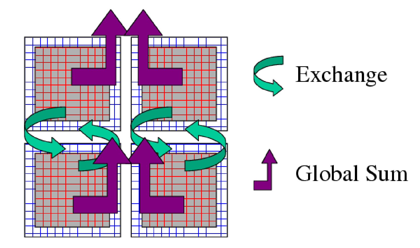
small number of communication primitives. Three optimizable primitives
are provided by the WRAPPER.
Figure 6.5 Three performance critical parallel primitives are provided by the WRAPPER. These primitives are always used to communicate data between tiles. The figure shows four tiles. The curved arrows indicate exchange primitives which transfer data between the overlap regions at tile edges and interior regions for nearest-neighbor tiles. The straight arrows symbolize global sum operations which connect all tiles. The global sum operation provides both a key arithmetic primitive and can serve as a synchronization primitive. A third barrier primitive is also provided, which behaves much like the global sum primitive.
EXCHANGE This operation is used to transfer data between interior
and overlap regions of neighboring tiles. A number of different forms
of this operation are supported. These different forms handle:
Data type differences. Sixty-four bit and thirty-two bit fields
may be handled separately.
Bindings to different communication methods. Exchange primitives
select between using shared memory or distributed memory
communication.
Transformation operations required when transporting data between
different grid regions. Transferring data between faces of a
cube-sphere grid, for example, involves a rotation of vector
components.
Forward and reverse mode computations. Derivative calculations
require tangent linear and adjoint forms of the exchange
primitives.
GLOBAL SUM The global sum operation is a central arithmetic
operation for the pressure inversion phase of the MITgcm algorithm.
For certain configurations, scaling can be highly sensitive to the
performance of the global sum primitive. This operation is a
collective operation involving all tiles of the simulated domain.
Different forms of the global sum primitive exist for handling:
Data type differences. Sixty-four bit and thirty-two bit fields
may be handled separately.
Bindings to different communication methods. Exchange primitives
select between using shared memory or distributed memory
communication.
Forward and reverse mode computations. Derivative calculations
require tangent linear and adjoint forms of the exchange
primitives.
BARRIER The WRAPPER provides a global synchronization function
called barrier. This is used to synchronize computations over all
tiles. The BARRIER and GLOBAL SUM primitives have much in
common and in some cases use the same underlying code.
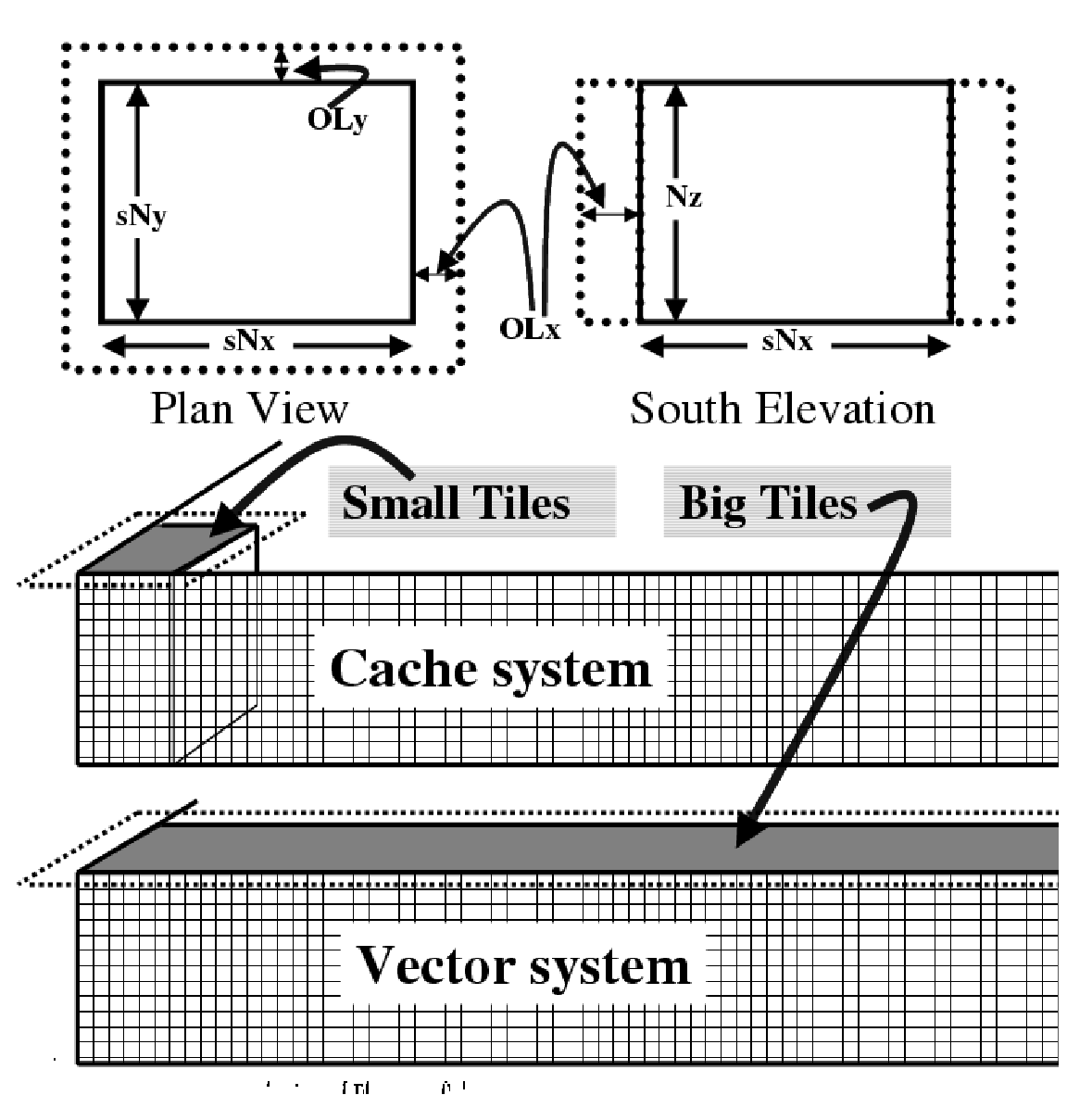
The WRAPPER machine model is aimed to target efficient systems with
highly pipelined memory architectures and systems with deep memory
hierarchies that favor memory reuse. This is achieved by supporting a
flexible tiling strategy as shown in Figure 6.6.
Within a CPU, computations are carried out sequentially on each tile in
turn. By reshaping tiles according to the target platform it is possible
to automatically tune code to improve memory performance. On a vector
machine a given domain might be subdivided into a few long, thin
regions. On a commodity microprocessor based system, however, the same
region could be simulated use many more smaller sub-domains.
Figure 6.6 The tiling strategy that the WRAPPER supports allows tiles to be shaped to suit the underlying system memory architecture. Compact tiles that lead to greater memory reuse can be used on cache based systems (upper half of figure) with deep memory hierarchies, whereas long tiles with large inner loops can be used to exploit vector systems having highly pipelined memory systems.
Following the discussion above, the machine model that the WRAPPER
presents to an application has the following characteristics:
The machine consists of one or more logical processors.
Each processor operates on tiles that it owns.
A processor may own more than one tile.
Processors may compute concurrently.
Exchange of information between tiles is handled by the machine
(WRAPPER) not by the application.
Behind the scenes this allows the WRAPPER to adapt the machine model
functions to exploit hardware on which:
Processors may be able to communicate very efficiently with each
other using shared memory.
An alternative communication mechanism based on a relatively simple
interprocess communication API may be required.
Shared memory may not necessarily obey sequential consistency,
however some mechanism will exist for enforcing memory consistency.
Memory consistency that is enforced at the hardware level may be
expensive. Unnecessary triggering of consistency protocols should be
avoided.
Memory access patterns may need to be either repetitive or highly
pipelined for optimum hardware performance.
This generic model, summarized in Figure 6.7, captures the essential hardware ingredients of almost
all successful scientific computer systems designed in the last 50
years.
In order to support maximum portability the WRAPPER is implemented
primarily in sequential Fortran 77. At a practical level the key steps
provided by the WRAPPER are:
specifying how a domain will be decomposed
starting a code in either sequential or parallel modes of operations
controlling communication between tiles and between concurrently
computing CPUs.
This section describes the details of each of these operations.
Section 6.3.1 explains the way a
domain is decomposed (or composed) is expressed. Section 6.3.2
describes practical details of running codes
in various different parallel modes on contemporary computer systems.
Section 6.3.3 explains the internal
information that the WRAPPER uses to control how information is
communicated between tiles.
At its heart, much of the WRAPPER works only in terms of a collection
of tiles which are interconnected to each other. This is also true of
application code operating within the WRAPPER. Application code is
written as a series of compute operations, each of which operates on a
single tile. If application code needs to perform operations involving
data associated with another tile, it uses a WRAPPER function to
obtain that data. The specification of how a global domain is
constructed from tiles or alternatively how a global domain is
decomposed into tiles is made in the file SIZE.h. This file defines
the following parameters:
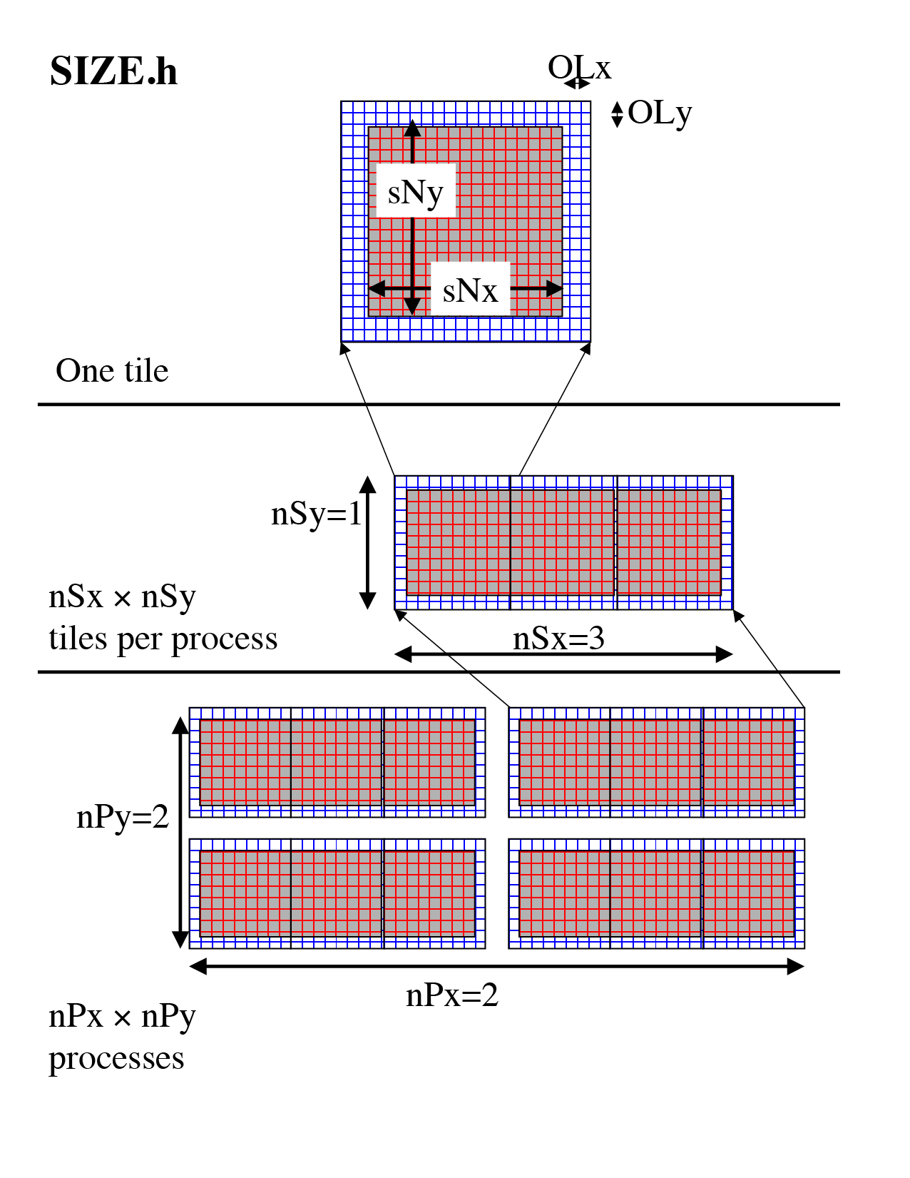
Together these parameters define a tiling decomposition of the style
shown in Figure 6.8. The parameters sNx and sNx
define the size of an individual tile. The parameters OLx and OLy
define the maximum size of the overlap extent. This must be set to the
maximum width of the computation stencil that the numerical code
finite-difference operations require between overlap region updates.
The maximum overlap required by any of the operations in the MITgcm
code distributed at this time is four grid points (some of the higher-order advection schemes
require a large overlap region). Code modifications and enhancements that involve adding wide
finite-difference stencils may require increasing OLx and OLy.
Setting OLx and OLy to a too large value will decrease code
performance (because redundant computations will be performed),
however it will not cause any other problems.
Figure 6.8 The three level domain decomposition hierarchy employed by the WRAPPER. A domain is composed of tiles. Multiple tiles can be allocated to a single process. Multiple processes can exist, each with multiple tiles. Tiles within a process can be spread over multiple compute threads.
The parameters nSx and nSy specify the number of tiles that will be
created within a single process. Each of these tiles will have internal
dimensions of sNx and sNy. If, when the code is executed, these
tiles are allocated to different threads of a process that are then
bound to different physical processors (see the multi-threaded
execution discussion in Section 6.3.2), then
computation will be performed concurrently on each tile. However, it is
also possible to run the same decomposition within a process running a
single thread on a single processor. In this case the tiles will be
computed over sequentially. If the decomposition is run in a single
process running multiple threads but attached to a single physical
processor, then, in general, the computation for different tiles will be
interleaved by system level software. This too is a valid mode of
operation.
The parameters sNx, sNy, OLx, OLy,
nSx and nSy are used extensively
by numerical code. The settings of sNx, sNy, OLx, and OLy are used to
form the loop ranges for many numerical calculations and to provide
dimensions for arrays holding numerical state. The nSx and nSy are
used in conjunction with the thread number parameter myThid. Much of
the numerical code operating within the WRAPPER takes the form:
The variables myBxLo(myThid), myBxHi(myThid), myByLo(myThid) and
myByHi(myThid) set the bounds of the loops in bi and bj in this
schematic. These variables specify the subset of the tiles in the range
1,nSx and 1,nSy1 that the logical processor bound to thread
number myThid owns. The thread number variable myThid ranges from 1
to the total number of threads requested at execution time. For each
value of myThid the loop scheme above will step sequentially through
the tiles owned by that thread. However, different threads will have
different ranges of tiles assigned to them, so that separate threads can
compute iterations of the bi, bj loop concurrently. Within a bi,
bj loop, computation is performed concurrently over as many processes
and threads as there are physical processors available to compute.
An exception to the the use of bi and bj in loops arises in the
exchange routines used when the exch2 package is used with the cubed
sphere. In this case bj is generally set to 1 and the loop runs from
1,bi. Within the loop bi is used to retrieve the tile number,
which is then used to reference exchange parameters.
The amount of computation that can be embedded in a single loop over bi
and bj varies for different parts of the MITgcm algorithm.
Consider a code extract from the 2-D implicit elliptic solver:
This portion of the code computes the \(L_2\)-Norm
of a vector whose elements are held in the array cg2d_r, writing the
final result to scalar variable err. Notice that under the WRAPPER,
arrays such as cg2d_r have two extra trailing dimensions. These right
most indices are tile indexes. Different threads with a single process
operate on different ranges of tile index, as controlled by the settings
of myByLo(myThid), myByHi(myThid), myBxLo(myThid) and
myBxHi(myThid). Because the \(L_2\)-Norm
requires a global reduction, the bi, bj loop above only contains one
statement. This computation phase is then followed by a communication
phase in which all threads and processes must participate. However, in
other areas of the MITgcm, code entries subsections of code are within a
single bi, bj loop. For example the evaluation of all the momentum
equation prognostic terms (see dynamics.F) is within a single
bi, bj loop.
The final decomposition parameters are nPx and nPy. These parameters
are used to indicate to the WRAPPER level how many processes (each with
nSx\(\times\)nSy tiles) will be used for this simulation.
This information is needed during initialization and during I/O phases.
However, unlike the variables sNx, sNy, OLx, OLy, nSx and nSy the
values of nPx and nPy are absent from the core numerical and support
code.
This sets up tiles with x-dimension of forty-five grid points,
y-dimension of twenty grid points, and x and y overlaps of three grid
points each. There are four tiles allocated to four separate
processes (nPx=2,nPy=2) and arranged so that the global domain size
is again ninety grid points in x and forty grid points in y. In
general the formula for global grid size (held in model variables
Nx and Ny) is
This sets up tiles with x-dimension of ninety grid points,
y-dimension of ten grid points, and x and y overlaps of three grid
points each. There are four tiles allocated to two separate processes
(nPy=2) each of which has two separate sub-domains nSy=2. The
global domain size is again ninety grid points in x and forty grid
points in y. The two sub-domains in each process will be computed
sequentially if they are given to a single thread within a single
process. Alternatively if the code is invoked with multiple threads
per process the two domains in y may be computed concurrently.
This sets up tiles with x-dimension of thirty-two grid points,
y-dimension of thirty-two grid points, and x and y overlaps of three
grid points each. There are six tiles allocated to six separate
logical processors (nSx=6). This set of values can be used for a
cube sphere calculation. Each tile of size \(32 \times 32\)
represents a face of the cube. Initializing the tile connectivity
correctly (see Section 6.3.3.3. allows the
rotations associated with moving between the six cube faces to be
embedded within the tile-tile communication code.
When code is started under the WRAPPER, execution begins in a main
routine eesupp/src/main.F that is owned by the WRAPPER. Control is
transferred to the application through a routine called
model/src/the_model_main.F once the WRAPPER has initialized correctly and has
created the necessary variables to support subsequent calls to
communication routines by the application code. The main stages of the WRAPPER startup calling
sequence are as follows:
Prior to transferring control to the procedure the_main_model.F
the WRAPPER may cause several coarse grain threads to be initialized.
The routine the_main_model.F is called once for each thread and is
passed a single stack argument which is the thread number, stored in
the myThid. In addition to specifying a decomposition with
multiple tiles per process (see Section 6.3.1) configuring and starting a code to
run using multiple threads requires the following steps.
First the code must be compiled with appropriate multi-threading
directives active in the file eesupp/src/main.F and with appropriate compiler
flags to request multi-threading support. The header files
eesupp/inc/MAIN_PDIRECTIVES1.h and eesupp/inc/MAIN_PDIRECTIVES2.h contain directives
compatible with compilers for Sun, Compaq, SGI, Hewlett-Packard SMP
systems and CRAY PVP systems. These directives can be activated by using
compile time directives -DTARGET_SUN, -DTARGET_DEC,
-DTARGET_SGI, -DTARGET_HP or -DTARGET_CRAY_VECTOR
respectively. Compiler options for invoking multi-threaded compilation
vary from system to system and from compiler to compiler. The options
will be described in the individual compiler documentation. For the
Fortran compiler from Sun the following options are needed to correctly
compile multi-threaded code
-stackvar -explicitpar -vpara -noautopar
These options are specific to the Sun compiler. Other compilers will use
different syntax that will be described in their documentation. The
effect of these options is as follows:
-stackvar Causes all local variables to be allocated in stack
storage. This is necessary for local variables to ensure that they
are private to their thread. Note, when using this option it may be
necessary to override the default limit on stack-size that the
operating system assigns to a process. This can normally be done by
changing the settings of the command shell’s stack-size.
However, on some systems changing this limit will require
privileged administrator access to modify system parameters.
-explicitpar Requests that multiple threads be spawned in
response to explicit directives in the application code. These
directives are inserted with syntax appropriate to the particular
target platform when, for example, the -DTARGET_SUN flag is
selected.
-vpara This causes the compiler to describe the multi-threaded
configuration it is creating. This is not required but it can be
useful when troubleshooting.
-noautopar This inhibits any automatic multi-threaded
parallelization the compiler may otherwise generate.
An example of valid settings for the eedata file for a domain with two
subdomains in y and running with two threads is shown below
nTx=1,nTy=2
This set of values will cause computations to stay within a single
thread when moving across the nSx sub-domains. In the y-direction,
however, sub-domains will be split equally between two threads.
Despite its appealing programming model, multi-threaded execution
remains less common than multi-process execution (described in Section 6.3.2.2).
One major reason for
this is that many system libraries are still not “thread-safe”. This
means that, for example, on some systems it is not safe to call system
routines to perform I/O when running in multi-threaded mode (except,
perhaps, in a limited set of circumstances). Another reason is that
support for multi-threaded programming models varies between systems.
Multi-process execution is more ubiquitous than multi-threaded execution.
In order to run code in a
multi-process configuration, a decomposition specification (see
Section 6.3.1) is given (in which at least one
of the parameters nPx or nPy will be greater than one). Then, as
for multi-threaded operation, appropriate compile time and run time
steps must be taken.
Multi-process execution under the WRAPPER assumes that portable,
MPI libraries are available for controlling the start-up of multiple
processes. The MPI libraries are not required, although they are
usually used, for performance critical communication. However, in
order to simplify the task of controlling and coordinating the start
up of a large number (hundreds and possibly even thousands) of copies
of the same program, MPI is used. The calls to the MPI multi-process
startup routines must be activated at compile time. Currently MPI
libraries are invoked by specifying the appropriate options file with
the -of flag when running the genmake2
script, which generates the
Makefile for compiling and linking MITgcm. (Previously this was done
by setting the ALLOW_USE_MPI and ALWAYS_USE_MPI flags in the
CPP_EEOPTIONS.h file.) More
detailed information about the use of
genmake2 for specifying local compiler
flags is located in Section 3.5.2.
The mechanics of starting a program in multi-process mode under MPI is
not standardized. Documentation associated with the distribution of MPI
installed on a system will describe how to start a program using that
distribution. For the open-source MPICH
system, the MITgcm program can
be started using a command such as
mpirun -np 64 -machinefile mf ./mitgcmuv
In this example the text -np64 specifies the number of processes
that will be created. The numeric value 64 must be equal to (or greater than) the
product of the processor grid settings of nPx and nPy in the file
SIZE.h. The option -machinefilemf
specifies that a text file called mf
will be read to get a list of processor names on which the sixty-four
processes will execute. The syntax of this file is specified by the
MPI distribution.
On some systems multi-threaded execution also requires the setting of a
special environment variable. On many machines this variable is called
PARALLEL and its values should be set to the number of parallel threads
required. Generally the help or manual pages associated with the
multi-threaded compiler on a machine will explain how to set the
required environment variables.
Finally the file eedata
needs to be configured to indicate the number
of threads to be used in the x and y directions:
# Example "eedata" file
# Lines beginning "#" are comments
# nTx - No. threads per process in X
# nTy - No. threads per process in Y
 &EEPARMS
 nTx=1,
 nTy=1,
 &
The product of nTx and nTy must be equal to the number of threads
spawned, i.e., the setting of the environment variable PARALLEL. The value
of nTx must subdivide the number of sub-domains in x (nSx) exactly.
The value of nTy must subdivide the number of sub-domains in y (nSy)
exactly. The multi-process startup of the MITgcm executable mitgcmuv is
controlled by the routines eeboot_minimal.F
and ini_procs.F. The
first routine performs basic steps required to make sure each process is
started and has a textual output stream associated with it. By default
two output files are opened for each process with names STDOUT.NNNN
and STDERR.NNNN. The NNNNN part of the name is filled in with
the process number so that process number 0 will create output files
STDOUT.0000 and STDERR.0000, process number 1 will create output
files STDOUT.0001 and STDERR.0001, etc. These files are used for
reporting status and configuration information and for reporting error
conditions on a process-by-process basis. The eeboot_minimal.F
procedure also sets the variables myProcId and MPI_COMM_MODEL.
These variables are related to processor identification and are used
later in the routine ini_procs.F to allocate tiles to processes.
Allocation of processes to tiles is controlled by the routine
ini_procs.F. For each process this routine sets the variables
myXGlobalLo and myYGlobalLo. These variables specify, in index
space, the coordinates of the southernmost and westernmost corner of
the southernmost and westernmost tile owned by this process. The
variables pidW, pidE, pidS and pidN are also set in this
routine. These are used to identify processes holding tiles to the
west, east, south and north of a given process. These values are
stored in global storage in the header file EESUPPORT.h for use by
communication routines. The above does not hold when the exch2 package
is used. The exch2 package sets its own parameters to specify the global
indices of tiles and their relationships to each other. See the
documentation on the exch2 package for details.
The WRAPPER maintains internal information that is used for
communication operations and can be customized for different
platforms. This section describes the information that is held and used.
Tile-tile connectivity information For each tile the WRAPPER sets
a flag that sets the tile number to the north, south, east and west
of that tile. This number is unique over all tiles in a
configuration. Except when using the cubed sphere and
the exch2 package,
the number is held in the variables tileNo (this holds
the tiles own number), tileNoN, tileNoS,
tileNoE and tileNoW.
A parameter is also stored with each tile that specifies the type of
communication that is used between tiles. This information is held in
the variables tileCommModeN, tileCommModeS,
tileCommModeE and
tileCommModeW. This latter set of variables can take one of the
following values COMM_NONE, COMM_MSG, COMM_PUT and
COMM_GET. A value of COMM_NONE is used to indicate that a tile
has no neighbor to communicate with on a particular face. A value of
COMM_MSG is used to indicate that some form of distributed memory
communication is required to communicate between these tile faces
(see Section 6.2.5.2). A value of
COMM_PUT or COMM_GET is used to indicate forms of shared memory
communication (see Section 6.2.5.1). The
COMM_PUT value indicates that a CPU should communicate by writing
to data structures owned by another CPU. A COMM_GET value
indicates that a CPU should communicate by reading from data
structures owned by another CPU. These flags affect the behavior of
the WRAPPER exchange primitive (see Figure 6.5). The routine
ini_communication_patterns.F
is responsible for setting the
communication mode values for each tile.
When using the cubed sphere configuration with the exch2 package, the
relationships between tiles and their communication methods are set
by the exch2 package and stored in different variables.
See the exch2 package
documentation for details.
MP directives The WRAPPER transfers control to numerical
application code through the routine
the_model_main.F. This routine
is called in a way that allows for it to be invoked by several
threads. Support for this is based on either multi-processing (MP)
compiler directives or specific calls to multi-threading libraries
(e.g., POSIX threads). Most commercially available Fortran compilers
support the generation of code to spawn multiple threads through some
form of compiler directives. Compiler directives are generally more
convenient than writing code to explicitly spawn threads. On
some systems, compiler directives may be the only method available.
The WRAPPER is distributed with template MP directives for a number
of systems.
These directives are inserted into the code just before and after the
transfer of control to numerical algorithm code through the routine
the_model_main.F. An example of
the code that performs this process for a Silicon Graphics system is as follows:
C--
C--  Parallel directives for MIPS Pro Fortran compiler
C--
C      Parallel compiler directives for SGI with IRIX
C$PAR  PARALLEL DO
C$PAR&  CHUNK=1,MP_SCHEDTYPE=INTERLEAVE,
C$PAR&  SHARE(nThreads),LOCAL(myThid,I)
C
      DO I=1,nThreads
        myThid = I

C--     Invoke nThreads instances of the numerical model
        CALL THE_MODEL_MAIN(myThid)

      ENDDO
Prior to transferring control to the procedure
the_model_main.F the
WRAPPER may use MP directives to spawn multiple threads. This code
is extracted from the files main.F and
eesupp/inc/MAIN_PDIRECTIVES1.h. The variable
nThreads specifies how many instances of the routine
the_model_main.F will be created.
The value of nThreads is set in the routine
ini_threading_environment.F.
The value is set equal to the the product of the parameters
nTx and nTy that are read from the file
eedata. If the value of nThreads is inconsistent with the number
of threads requested from the operating system (for example by using
an environment variable as described in Section 6.3.2.1)
then usually an error will be
reported by the routine check_threads.F.
memsync flags As discussed in Section 6.2.5.1,
a low-level system function may be need to force memory consistency
on some shared memory systems. The routine
memsync.F is used for
this purpose. This routine should not need modifying and the
information below is only provided for completeness. A logical
parameter exchNeedsMemSync set in the routine
ini_communication_patterns.F
controls whether the memsync.F
primitive is called. In general this routine is only used for
multi-threaded execution. The code that goes into the memsync.F
routine is specific to the compiler and processor used. In some
cases, it must be written using a short code snippet of assembly
language. For an Ultra Sparc system the following code snippet is
used
asm("membar #LoadStore|#StoreStore");
For an Alpha based system the equivalent code reads
asm("mb");
while on an x86 system the following code is required
asm("lock; addl $0,0(%%esp)": : :"memory")
Cache line size As discussed in Section 6.2.5.1,
multi-threaded codes
explicitly avoid penalties associated with excessive coherence
traffic on an SMP system. To do this the shared memory data
structures used by the global_sum.F,
global_max.F and
barrier.F
routines are padded. The variables that control the padding are set
in the header file EEPARAMS.h.
These variables are called cacheLineSize, lShare1,
lShare4 and lShare8. The default
values should not normally need changing.
_BARRIER This is a CPP macro that is expanded to a call to a
routine which synchronizes all the logical processors running under
the WRAPPER. Using a macro here preserves flexibility to insert a
specialized call in-line into application code. By default this
resolves to calling the procedure barrier.F.
The default setting for the _BARRIER macro is given in the
file CPP_EEMACROS.h.
_GSUM This is a CPP macro that is expanded to a call to a
routine which sums up a floating point number over all the logical
processors running under the WRAPPER. Using a macro here provides
extra flexibility to insert a specialized call in-line into
application code. By default this resolves to calling the procedure
GLOBAL_SUM_R8() for 64-bit floating point operands or
GLOBAL_SUM_R4() for 32-bit floating point operand
(located in file global_sum.F). The default
setting for the _GSUM macro is given in the file
CPP_EEMACROS.h.
The _GSUM macro is a performance critical operation, especially for
large processor count, small tile size configurations. The custom
communication example discussed in Section 6.3.3.2 shows
how the macro is used to invoke a custom global sum routine for a
specific set of hardware.
_EXCH The _EXCH CPP macro is used to update tile overlap
regions. It is qualified by a suffix indicating whether overlap
updates are for two-dimensional (_EXCH_XY) or three dimensional
(_EXCH_XYZ) physical fields and whether fields are 32-bit floating
point (_EXCH_XY_R4, _EXCH_XYZ_R4) or 64-bit floating point
(_EXCH_XY_R8, _EXCH_XYZ_R8). The macro mappings are defined in
the header file CPP_EEMACROS.h.
As with _GSUM, the _EXCH
operation plays a crucial role in scaling to small tile, large
logical and physical processor count configurations. The example in
Section 6.3.3.2 discusses defining an optimized and
specialized form on the _EXCH operation.
The _EXCH operation is also central to supporting grids such as the
cube-sphere grid. In this class of grid a rotation may be required
between tiles. Aligning the coordinate requiring rotation with the
tile decomposition allows the coordinate transformation to be
embedded within a custom form of the _EXCH primitive. In these cases
_EXCH is mapped to exch2 routines, as detailed in the exch2 package
documentation.
Reverse Mode The communication primitives _EXCH and _GSUM both
employ hand-written adjoint forms (or reverse mode) forms. These
reverse mode forms can be found in the source code directory
pkg/autodiff. For the global sum primitive the reverse mode form
calls are to GLOBAL_ADSUM_R4() and GLOBAL_ADSUM_R8() (located in
file global_sum_ad.F). The reverse
mode form of the exchange primitives are found in routines prefixed
ADEXCH. The exchange routines make calls to the same low-level
communication primitives as the forward mode operations. However, the
routine argument theSimulationMode is set to the value
REVERSE_SIMULATION. This signifies to the low-level routines that
the adjoint forms of the appropriate communication operation should
be performed.
MAX_NO_THREADS The variable MAX_NO_THREADS is used to
indicate the maximum number of OS threads that a code will use. This
value defaults to thirty-two and is set in the file
EEPARAMS.h. For
single threaded execution it can be reduced to one if required. The
value is largely private to the WRAPPER and application code will not
normally reference the value, except in the following scenario.
For certain physical parametrization schemes it is necessary to have
a substantial number of work arrays. Where these arrays are allocated
in heap storage (for example COMMON blocks) multi-threaded execution
will require multiple instances of the COMMON block data. This can be
achieved using a Fortran 90 module construct. However, if this
mechanism is unavailable then the work arrays can be extended with
dimensions using the tile dimensioning scheme of nSx and nSy (as
described in Section 6.3.1). However, if
the configuration being specified involves many more tiles than OS
threads then it can save memory resources to reduce the variable
MAX_NO_THREADS to be equal to the actual number of threads that
will be used and to declare the physical parameterization work arrays
with a single MAX_NO_THREADS extra dimension. An example of this
is given in the verification experiment verification/aim.5l_cs. Here the
default setting of MAX_NO_THREADS is altered to
and several work arrays for storing intermediate calculations are
created with declarations of the form.
common /FORCIN/ sst1(ngp,MAX_NO_THREADS)
This declaration scheme is not used widely, because most global data
is used for permanent, not temporary, storage of state information. In
the case of permanent state information this approach cannot be used
because there has to be enough storage allocated for all tiles.
However, the technique can sometimes be a useful scheme for reducing
memory requirements in complex physical parameterizations.
The isolation of performance critical communication primitives and the
subdivision of the simulation domain into tiles is a powerful tool.
Here we show how it can be used to improve application performance and
how it can be used to adapt to new gridding approaches.
On some platforms a big performance boost can be obtained by binding the
communication routines _EXCH and _GSUM to specialized native
libraries (for example, the shmem library on CRAY T3E systems). The
LETS_MAKE_JAM CPP flag is used as an illustration of a specialized
communication configuration that substitutes for standard, portable
forms of _EXCH and _GSUM. It affects three source files
eeboot.F, CPP_EEMACROS.h
and cg2d.F. When the flag is defined is
has the following effects.
An extra phase is included at boot time to initialize the custom
communications library (see ini_jam.F).
The _GSUM and _EXCH macro definitions are replaced with calls
to custom routines (see gsum_jam.F and exch_jam.F)
a highly specialized form of the exchange operator (optimized for
overlap regions of width one) is substituted into the elliptic solver
routine cg2d.F.
Developing specialized code for other libraries follows a similar
pattern.
Actual _EXCH routine code is generated automatically from a series of
template files, for example
exch2_rx1_cube.template.
This is done to allow a
large number of variations of the exchange process to be maintained. One
set of variations supports the cube sphere grid. Support for a cube
sphere grid in MITgcm is based on having each face of the cube as a
separate tile or tiles. The exchange routines are then able to absorb
much of the detailed rotation and reorientation required when moving
around the cube grid. The set of _EXCH routines that contain the word
cube in their name perform these transformations. They are invoked when
the run-time logical parameter useCubedSphereExchange is
set .TRUE.. To
facilitate the transformations on a staggered C-grid, exchange
operations are defined separately for both vector and scalar quantities
and for grid-centered and for grid-face and grid-corner quantities.
Three sets of exchange routines are defined. Routines with names of the
form exch2_rx are used to exchange cell centered scalar quantities.
Routines with names of the form exch2_uv_rx are used to exchange
vector quantities located at the C-grid velocity points. The vector
quantities exchanged by the exch_uv_rx routines can either be signed
(for example velocity components) or un-signed (for example grid-cell
separations). Routines with names of the form exch_z_rx are used to
exchange quantities at the C-grid vorticity point locations.
Fitting together the WRAPPER elements, package elements and MITgcm core
equation elements of the source code produces the calling sequence shown below.
6.4.1. Annotated call tree for MITgcm and WRAPPER