This chapter lays out the numerical schemes that are employed in the
core MITgcm algorithm. Whenever possible links are made to actual
program code in the MITgcm implementation. The chapter begins with a
discussion of the temporal discretization used in MITgcm. This
discussion is followed by sections that describe the spatial
discretization. The schemes employed for momentum terms are described
first, afterwards the schemes that apply to passive and dynamically
active tracers are described.
Because of the particularity of the vertical direction in stratified
fluid context, in this chapter, the vector notations are mostly used for
the horizontal component: the horizontal part of a vector is simply
written \(\vec{\bf v}\) (instead of \({{\bf v}_h}\) or
\(\vec{\mathbf{v}}_{h}\) in chapter 1) and a 3D vector is simply
written \(\vec{v}\) (instead of \(\vec{\mathbf{v}}\) in chapter
1).
The notations we use to describe the discrete formulation of the model
are summarized as follows.
General notation:
\(\Delta x, \Delta y, \Delta r\) grid spacing in X, Y, R directions
\(A_c,A_w,A_s,A_{\zeta}\) : horizontal area of a grid cell surrounding \(\theta,u,v,\zeta\) point
\({\cal V}_u , {\cal V}_v , {\cal V}_w , {\cal V}_\theta\) : Volume of the grid box surrounding \(u,v,w,\theta\) point
\(i,j,k\) : current index relative to X, Y, R directions
The equations of motion integrated by the model involve four prognostic
equations for flow, \(u\) and \(v\), temperature,
\(\theta\), and salt/moisture, \(S\), and three diagnostic
equations for vertical flow, \(w\), density/buoyancy,
\(\rho\)/\(b\), and pressure/geo-potential, \(\phi_{\rm hyd}\).
In addition, the surface pressure or height may by described by either a
prognostic or diagnostic equation and if non-hydrostatics terms are
included then a diagnostic equation for non-hydrostatic pressure is also
solved. The combination of prognostic and diagnostic equations requires
a model algorithm that can march forward prognostic variables while
satisfying constraints imposed by diagnostic equations.
Since the model comes in several flavors and formulation, it would be
confusing to present the model algorithm exactly as written into code
along with all the switches and optional terms. Instead, we present the
algorithm for each of the basic formulations which are:
the semi-implicit pressure method for hydrostatic equations with a
rigid-lid, variables co-located in time and with Adams-Bashforth
time-stepping;
as 1 but with an implicit linear free-surface;
as 1 or 2 but with variables staggered in time;
as 1 or 2 but with non-hydrostatic terms included;
as 2 or 3 but with non-linear free-surface.
In all the above configurations it is also possible to substitute the
Adams-Bashforth with an alternative time-stepping scheme for terms
evaluated explicitly in time. Since the over-arching algorithm is
independent of the particular time-stepping scheme chosen we will
describe first the over-arching algorithm, known as the pressure method,
with a rigid-lid model in Section 2.3. This
algorithm is essentially unchanged, apart for some coefficients, when
the rigid lid assumption is replaced with a linearized implicit
free-surface, described in Section 2.4. These two flavors of the
pressure-method encompass all formulations of the model as it exists
today. The integration of explicit in time terms is out-lined in
Section 2.5 and put into the context of the overall algorithm
in Section 2.7 and Section 2.8.
Inclusion of non-hydrostatic terms
requires applying the pressure method in three dimensions instead of two
and this algorithm modification is described in
Section 2.9. Finally, the free-surface equation may be treated
more exactly, including non-linear terms, and this is described in
Section 2.10.2.
The horizontal momentum and continuity equations for the ocean
((1.98) and (1.100)), or for the atmosphere
((1.45) and (1.47)), can be summarized by:
\[\begin{split}\begin{aligned}
\partial_t u + g \partial_x \eta & = G_u \\
\partial_t v + g \partial_y \eta & = G_v \\
\partial_x u + \partial_y v + \partial_z w & = 0\end{aligned}\end{split}\]
where we are adopting the oceanic notation for brevity. All terms in
the momentum equations, except for surface pressure gradient, are
encapsulated in the \(G\) vector. The continuity equation, when
integrated over the fluid depth, \(H\), and with the rigid-lid/no
normal flow boundary conditions applied, becomes:
(2.1)\[\partial_x H \widehat{u} + \partial_y H \widehat{v} = 0\]
Here, \(H\widehat{u} = \int_H u dz\) is the depth integral of
\(u\), similarly for \(H\widehat{v}\). The rigid-lid
approximation sets \(w=0\) at the lid so that it does not move but
allows a pressure to be exerted on the fluid by the lid. The horizontal
momentum equations and vertically integrated continuity equation are be
discretized in time and space as follows:
(2.2)\[u^{n+1} + \Delta t g \partial_x \eta^{n+1}
= u^{n} + \Delta t G_u^{(n+1/2)}\]
(2.3)\[v^{n+1} + \Delta t g \partial_y \eta^{n+1}
= v^{n} + \Delta t G_v^{(n+1/2)}\]
(2.4)\[\partial_x H \widehat{u^{n+1}}
+ \partial_y H \widehat{v^{n+1}} = 0\]
As written here, terms on the LHS all involve time level \(n+1\)
and are referred to as implicit; the implicit backward time stepping
scheme is being used. All other terms in the RHS are explicit in time.
The thermodynamic quantities are integrated forward in time in parallel
with the flow and will be discussed later. For the purposes of
describing the pressure method it suffices to say that the hydrostatic
pressure gradient is explicit and so can be included in the vector
\(G\).
Substituting the two momentum equations into the depth-integrated
continuity equation eliminates \(u^{n+1}\) and \(v^{n+1}\)
yielding an elliptic equation for \(\eta^{n+1}\). Equations
(2.2), (2.3) and
(2.4) can then be re-arranged as follows:
(2.7)\[\partial_x \Delta t g H \partial_x \eta^{n+1}
+ \partial_y \Delta t g H \partial_y \eta^{n+1}
= \partial_x H \widehat{u^{*}}
+ \partial_y H \widehat{v^{*}}\]
(2.8)\[u^{n+1} = u^{*} - \Delta t g \partial_x \eta^{n+1}\]
(2.9)\[v^{n+1} = v^{*} - \Delta t g \partial_y \eta^{n+1}\]
Equations (2.5) to (2.9), solved
sequentially, represent the pressure method algorithm used in the model.
The essence of the pressure method lies in the fact that any explicit
prediction for the flow would lead to a divergence flow field so a
pressure field must be found that keeps the flow non-divergent over each
step of the integration. The particular location in time of the pressure
field is somewhat ambiguous; in Figure 2.1 we
depicted as co-located with the future flow field (time level
\(n+1\)) but it could equally have been drawn as staggered in time
with the flow.
Figure 2.1 A schematic of the evolution in time of the pressure method algorithm. A prediction for the flow variables at time level \(n+1\) is made based only on the explicit terms, \(G^{(n+^1/_2)}\), and denoted \(u^*\), \(v^*\). Next, a pressure field is found such that \(u^{n+1}\), \(v^{n+1}\) will be non-divergent. Conceptually, the \(*\) quantities exist at time level \(n+1\) but they are intermediate and only temporary.
The correspondence to the code is as follows:
the prognostic phase, equations (2.5) and
(2.6), stepping forward \(u^n\) and \(v^n\) to
\(u^{*}\) and \(v^{*}\) is coded in timestep.F
the vertical integration, \(H \widehat{u^*}\) and \(H
\widehat{v^*}\), divergence and inversion of the elliptic operator in
equation (2.7) is coded in solve_for_pressure.F
finally, the new flow field at time level \(n+1\) given by
equations (2.8) and (2.9) is calculated
in correction_step.F
The calling tree for these routines is as follows:
In general, the horizontal momentum time-stepping can contain some terms
that are treated implicitly in time, such as the vertical viscosity when
using the backward time-stepping scheme (implicitViscosity=.TRUE.). The method used to solve
those implicit terms is provided in Section 2.6, and modifies equations
(2.2) and (2.3) to give:
\[\begin{split}\begin{aligned}
u^{n+1} - \Delta t \partial_z A_v \partial_z u^{n+1}
+ \Delta t g \partial_x \eta^{n+1} & = u^{n} + \Delta t G_u^{(n+1/2)}
\\
v^{n+1} - \Delta t \partial_z A_v \partial_z v^{n+1}
+ \Delta t g \partial_y \eta^{n+1} & = v^{n} + \Delta t G_v^{(n+1/2)}\end{aligned}\end{split}\]
2.4. Pressure method with implicit linear free-surface
The rigid-lid approximation filters out external gravity waves
subsequently modifying the dispersion relation of barotropic Rossby
waves. The discrete form of the elliptic equation has some zero
eigenvalues which makes it a potentially tricky or inefficient problem
to solve.
The rigid-lid approximation can be easily replaced by a linearization of
the free-surface equation which can be written:
(2.10)\[\partial_t \eta + \partial_x H \widehat{u} + \partial_y H \widehat{v} = {\mathcal{P-E+R}}\]
which differs from the depth-integrated continuity equation with
rigid-lid (2.1) by the time-dependent term and
fresh-water source term.
Equation (2.4) in the rigid-lid pressure
method is then replaced by the time discretization of
(2.10) which is:
(2.11)\[\eta^{n+1}
+ \Delta t \partial_x H \widehat{u^{n+1}}
+ \Delta t \partial_y H \widehat{v^{n+1}}
= \eta^{n} + \Delta t ( {\mathcal{P-E}})\]
where the use of flow at time level \(n+1\) makes the method
implicit and backward in time. This is the preferred scheme since it
still filters the fast unresolved wave motions by damping them. A
centered scheme, such as Crank-Nicolson (see
Section 2.10.1), would alias the energy of the fast modes onto
slower modes of motion.
As for the rigid-lid pressure method, equations (2.2),
(2.3) and (2.11) can be
re-arranged as follows:
(2.14)\[\eta^* = \epsilon_{\rm fs} ( \eta^{n} + \Delta t ({\mathcal{P-E}}) )
- \Delta t ( \partial_x H \widehat{u^{*}}
+ \partial_y H \widehat{v^{*}} )\]
(2.15)\[\partial_x g H \partial_x \eta^{n+1}
+ \partial_y g H \partial_y \eta^{n+1}
- \frac{\epsilon_{\rm fs} \eta^{n+1}}{\Delta t^2} =
- \frac{\eta^*}{\Delta t^2}\]
(2.16)\[u^{n+1} = u^{*} - \Delta t g \partial_x \eta^{n+1}\]
(2.17)\[v^{n+1} = v^{*} - \Delta t g \partial_y \eta^{n+1}\]
Equations (2.12)
to (2.17), solved sequentially, represent the
pressure method algorithm with a backward implicit, linearized free
surface. The method is still formerly a pressure method because in the
limit of large \(\Delta t\) the rigid-lid method is recovered.
However, the implicit treatment of the free-surface allows the flow to
be divergent and for the surface pressure/elevation to respond on a
finite time-scale (as opposed to instantly). To recover the rigid-lid
formulation, we use a switch-like variable,
\(\epsilon_{\rm fs}\) (freesurfFac), which selects between the free-surface and
rigid-lid; \(\epsilon_{\rm fs}=1\) allows the free-surface to evolve;
\(\epsilon_{\rm fs}=0\) imposes the rigid-lid. The evolution in time and
location of variables is exactly as it was for the rigid-lid model so
that Figure 2.1 is still applicable.
Similarly, the calling sequence, given here, is as for the pressure-method.
In describing the the pressure method above we deferred describing the
time discretization of the explicit terms. We have historically used the
quasi-second order Adams-Bashforth method (AB-II) for all explicit terms in both
the momentum and tracer equations. This is still the default mode of
operation but it is now possible to use alternate schemes for tracers
(see Section 2.16), or a 3rd order Adams-Bashforth method (AB-III).
In the previous sections, we summarized an explicit scheme as:
(2.18)\[\tau^{*} = \tau^{n} + \Delta t G_\tau^{(n+1/2)}\]
where \(\tau\) could be any prognostic variable (\(u\),
\(v\), \(\theta\) or \(S\)) and \(\tau^*\) is an
explicit estimate of \(\tau^{n+1}\) and would be exact if not for
implicit-in-time terms. The parenthesis about \(n+1/2\) indicates
that the term is explicit and extrapolated forward in time. Below we describe
in more detail the AB-II and AB-III schemes.
This is a linear extrapolation, forward in time, to
\(t=(n+1/2+{\epsilon_{\rm AB}})\Delta t\). An extrapolation to the
mid-point in time, \(t=(n+1/2)\Delta t\), corresponding to
\(\epsilon_{\rm AB}=0\), would be second order accurate but is weakly
unstable for oscillatory terms. A small but finite value for
\(\epsilon_{\rm AB}\) stabilizes the method. Strictly speaking, damping
terms such as diffusion and dissipation, and fixed terms (forcing), do
not need to be inside the Adams-Bashforth extrapolation. However, in the
current code, it is simpler to include these terms and this can be
justified if the flow and forcing evolves smoothly. Problems can, and
do, arise when forcing or motions are high frequency and this
corresponds to a reduced stability compared to a simple forward
time-stepping of such terms. The model offers the possibility to leave
terms outside the Adams-Bashforth extrapolation, by turning off the logical flag forcing_In_AB
(parameter file data, namelist PARM01, default value = .TRUE.) and then setting tracForcingOutAB
(default=0), momForcingOutAB (default=0), and momDissip_In_AB (parameter file data, namelist PARM01,
default value = TRUE), respectively for the tracer terms, momentum forcing terms, and the dissipation terms.
A stability analysis for an oscillation equation should be given at this
point.
A stability analysis for a relaxation equation should be given at this
point.
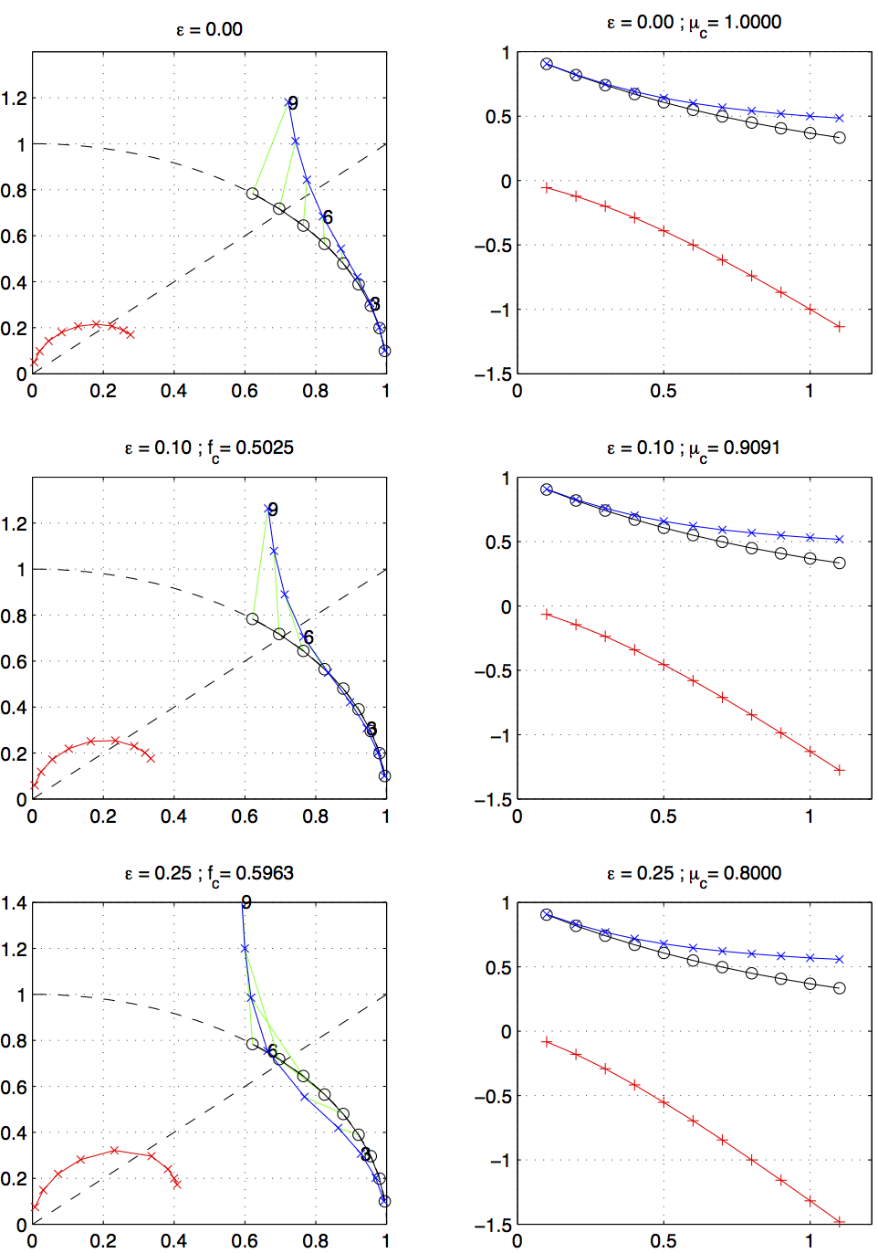
Figure 2.2 Oscillatory and damping response of quasi-second order Adams-Bashforth scheme for different values of the \(\epsilon _{\rm AB}\)
parameter (0.0, 0.1, 0.25, from top to bottom) The analytical solution (in black), the physical mode (in blue) and the numerical
mode (in red) are represented with a CFL step of 0.1. The left column represents the oscillatory response on the complex plane
for CFL ranging from 0.1 up to 0.9. The right column represents the damping response amplitude (y-axis) function of the CFL (x-axis).
The 3rd order Adams-Bashforth time stepping (AB-III) provides several
advantages (see, e.g., Durran 1991 [Dur91]) compared to the
default quasi-second order Adams-Bashforth method:
higher accuracy;
stable with a longer time-step;
no additional computation (just requires the storage of one
additional time level).
The 3rd order Adams-Bashforth can be used to extrapolate
forward in time the tendency (replacing (2.19))
as:
3rd order accuracy is obtained with
\((\alpha_{\rm AB},\,\beta_{\rm AB}) = (1/2,\,5/12)\). Note that selecting
\((\alpha_{\rm AB},\,\beta_{\rm AB}) = (1/2+\epsilon_{AB},\,0)\) one
recovers AB-II. The AB-III time stepping improves the
stability limit for an oscillatory problem like advection or Coriolis.
As seen from Figure 2.3, it remains stable up to a
CFL of 0.72, compared to only 0.50 with AB-II and
\(\epsilon_{\rm AB} = 0.1\). It is interesting to note that the
stability limit can be further extended up to a CFL of 0.786 for an
oscillatory problem (see Figure 2.3) using
\((\alpha_{\rm AB},\,\beta_{\rm AB}) = (0.5,\,0.2811)\) but then the scheme
is only second order accurate.
However, the behavior of the AB-III for a damping problem (like diffusion)
is less favorable, since the stability limit is reduced to 0.54 only
(and 0.64 with \(\beta_{\rm AB} = 0.2811\)) compared to 1.0 (and 0.9 with
\(\epsilon_{\rm AB} = 0.1\)) with the AB-II (see
Figure 2.4).
A way to enable the use of a longer time step is to keep the dissipation
terms outside the AB extrapolation (setting momDissip_In_AB to .FALSE.
in main parameter file data, namelist PARM03, thus returning to
a simple forward time-stepping for dissipation, and to use AB-III only for
advection and Coriolis terms.
The AB-III time stepping is activated by defining the option #defineALLOW_ADAMSBASHFORTH_3 in CPP_OPTIONS.h. The parameters
\(\alpha_{\rm AB},\beta_{\rm AB}\) can be set from the main parameter file
data (namelist PARM03) and their default values correspond to
the 3rd order Adams-Bashforth. A simple example is provided in
verification/advect_xy/input.ab3_c4.
AB-III is not yet available for the vertical momentum equation
(non-hydrostatic) nor for passive tracers.
Figure 2.3 Oscillatory response of third order Adams-Bashforth scheme for different values of the \((\alpha_{\rm AB},\,\beta_{\rm AB})\) parameters.
The analytical solution (in black), the physical mode (in blue) and the numerical mode (in red) are represented with a CFL step of 0.1.
Figure 2.4 Damping response of third order Adams-Bashforth scheme for different values of the \((\alpha_{\rm AB},\,\beta_{\rm AB})\) parameters.
The analytical solution (in black), the physical mode (in blue) and the numerical mode (in red) are represented with a CFL step of 0.1.
Vertical diffusion and viscosity can be treated implicitly in time using
the backward method which is an intrinsic scheme. Recently, the option
to treat the vertical advection implicitly has been added, but not yet
tested; therefore, the description hereafter is limited to diffusion and
viscosity. For tracers, the time discretized equation is:
(2.21)\[\tau^{n+1} - \Delta t \partial_r \kappa_v \partial_r \tau^{n+1} = \tau^{n} + \Delta t G_\tau^{(n+1/2)}\]
where \(G_\tau^{(n+1/2)}\) is the remaining explicit terms
extrapolated using the Adams-Bashforth method as described above.
Equation (2.21) can be split split into:
(2.22)\[\tau^* = \tau^{n} + \Delta t G_\tau^{(n+1/2)}\]
Equation (2.22) looks exactly as (2.18) while
(2.23) involves an operator or matrix inversion. By
re-arranging (2.21) in this way we have cast the method
as an explicit prediction step and an implicit step allowing the latter
to be inserted into the over all algorithm with minimal interference.
The calling sequence for stepping forward a tracer variable such as temperature with implicit diffusion is
as follows:
In order to fit within the pressure method, the implicit viscosity must
not alter the barotropic flow. In other words, it can only redistribute
momentum in the vertical. The upshot of this is that although vertical
viscosity may be backward implicit and unconditionally stable, no-slip
boundary conditions may not be made implicit and are thus cast as a an
explicit drag term.
2.7. Synchronous time-stepping: variables co-located in time
Figure 2.5 A schematic of the explicit Adams-Bashforth and implicit time-stepping phases of the algorithm. All prognostic variables are co-located in time. Explicit tendencies are evaluated at time level \(n\) as a function of the state at that time level (dotted arrow). The explicit tendency from the previous time level, \(n-1\), is used to extrapolate tendencies to \(n+1/2\) (dashed arrow). This extrapolated tendency allows variables to be stably integrated forward-in-time to render an estimate (\(*\) -variables) at the \(n+1\) time level (solid arc-arrow). The operator \({\cal L}\) formed from implicit-in-time terms is solved to yield the state variables at time level \(n+1\).
The Adams-Bashforth extrapolation of explicit tendencies fits neatly
into the pressure method algorithm when all state variables are
co-located in time. The algorithm can be represented by the sequential solution of the
follow equations:
(2.33)\[\eta^* = \epsilon_{\rm fs} \left( \eta^{n} + \Delta t ({\mathcal{P-E}}) \right)- \Delta t
\nabla \cdot H \widehat{ \vec{\bf v}^{**} }\]
(2.34)\[\nabla \cdot g H \nabla \eta^{n+1} - \frac{\epsilon_{\rm fs} \eta^{n+1}}{\Delta t^2} ~ = ~ - \frac{\eta^*}{\Delta t^2}\]
(2.35)\[\vec{\bf v}^{n+1} = \vec{\bf v}^{**} - \Delta t g \nabla \eta^{n+1}\]
Figure 2.5 illustrates the location of variables
in time and evolution of the algorithm with time. The Adams-Bashforth
extrapolation of the tracer tendencies is illustrated by the dashed
arrow, the prediction at \(n+1\) is indicated by the solid arc.
Inversion of the implicit terms, \({\cal
L}^{-1}_{\theta,S}\), then yields the new tracer fields at \(n+1\).
All these operations are carried out in subroutine THERMODYNAMICS and
subsidiaries, which correspond to equations (2.24) to
(2.27). Similarly illustrated is the Adams-Bashforth
extrapolation of accelerations, stepping forward and solving of implicit
viscosity and surface pressure gradient terms, corresponding to
equations (2.29) to (2.35). These operations are
carried out in subroutines DYNAMICS,
SOLVE_FOR_PRESSURE and
MOMENTUM_CORRECTION_STEP.
This, then, represents an entire algorithm
for stepping forward the model one time-step. The corresponding calling
tree for the overall synchronous algorithm using
Adams-Bashforth time-stepping is given below. The place where the model geometry
hFac factors) is updated is added here but is only relevant
for the non-linear free-surface algorithm.
For completeness, the external forcing,
ocean and atmospheric physics have been added, although they are mainly optional.
Figure 2.6 A schematic of the explicit Adams-Bashforth and implicit time-stepping phases of the algorithm but with staggering in time of thermodynamic variables with the flow. Explicit momentum tendencies are evaluated at time level \(n-1/2\) as a function of the flow field at that time level \(n-1/2\). The explicit tendency from the previous time level, \(n-3/2\), is used to extrapolate tendencies to \(n\) (dashed arrow). The hydrostatic pressure/geo-potential \(\phi _{\rm hyd}\) is evaluated directly at time level \(n\) (vertical arrows) and used with the extrapolated tendencies to step forward the flow variables from \(n-1/2\) to \(n+1/2\) (solid arc-arrow). The implicit-in-time operator \({\cal L}_{\bf u,v}\) (vertical arrows) is then applied to the previous estimation of the the flow field (\(*\) -variables) and yields to the two velocity components \(u,v\) at time level \(n+1/2\). These are then used to calculate the advection term (dashed arc-arrow) of the thermo-dynamics tendencies at time step \(n\). The extrapolated thermodynamics tendency, from time level \(n-1\) and \(n\) to \(n+1/2\), allows thermodynamic variables to be stably integrated forward-in-time (solid arc-arrow) up to time level \(n+1\).
For well-stratified problems, internal gravity waves may be the limiting
process for determining a stable time-step. In the circumstance, it is
more efficient to stagger in time the thermodynamic variables with the
flow variables. Figure 2.6 illustrates the
staggering and algorithm. The key difference between this and
Figure 2.5 is that the thermodynamic variables are
solved after the dynamics, using the recently updated flow field. This
essentially allows the gravity wave terms to leap-frog in time giving
second order accuracy and more stability.
The essential change in the staggered algorithm is that the
thermodynamics solver is delayed from half a time step, allowing the use
of the most recent velocities to compute the advection terms. Once the
thermodynamics fields are updated, the hydrostatic pressure is computed
to step forward the dynamics. Note that the pressure gradient must also
be taken out of the Adams-Bashforth extrapolation. Also, retaining the
integer time-levels, \(n\) and \(n+1\), does not give a user the
sense of where variables are located in time. Instead, we re-write the
entire algorithm, (2.24) to (2.35), annotating the
position in time of variables appropriately:
The corresponding calling tree is given below. The staggered algorithm is
activated with the run-time flag staggerTimeStep=.TRUE. in
parameter file data, namelist PARM01.
The only difficulty with this approach is apparent in equation
(2.44) and illustrated by the dotted arrow connecting
\(u,v^{n+1/2}\) with \(G_\theta^{n}\). The flow used to advect
tracers around is not naturally located in time. This could be avoided
by applying the Adams-Bashforth extrapolation to the tracer field itself
and advecting that around but this approach is not yet available. We’re
not aware of any detrimental effect of this feature. The difficulty lies
mainly in interpretation of what time-level variables and terms
correspond to.
The non-hydrostatic formulation re-introduces the full vertical momentum
equation and requires the solution of a 3-D elliptic equations for
non-hydrostatic pressure perturbation. We still integrate vertically for
the hydrostatic pressure and solve a 2-D elliptic equation for the
surface pressure/elevation for this reduces the amount of work needed to
solve for the non-hydrostatic pressure.
The momentum equations are discretized in time as follows:
As before, the explicit predictions for momentum are consolidated as:
\[\begin{split}\begin{aligned}
u^* & = u^n + \Delta t G_u^{(n+1/2)} \\
v^* & = v^n + \Delta t G_v^{(n+1/2)} \\
w^* & = w^n + \Delta t G_w^{(n+1/2)}\end{aligned}\end{split}\]
but this time we introduce an intermediate step by splitting the
tendency of the flow as follows:
\[\begin{split}\begin{aligned}
u^{n+1} = u^{**} - \Delta t \partial_x \phi_{\rm nh}^{n+1}
& &
u^{**} = u^{*} - \Delta t g \partial_x \eta^{n+1} \\
v^{n+1} = v^{**} - \Delta t \partial_y \phi_{\rm nh}^{n+1}
& &
v^{**} = v^{*} - \Delta t g \partial_y \eta^{n+1}\end{aligned}\end{split}\]
Substituting into the depth integrated continuity
(2.11) gives
(2.52)\[\partial_x H \partial_x \left( g \eta^{n+1} + \widehat{\phi}_{\rm nh}^{n+1} \right)
+ \partial_y H \partial_y \left( g \eta^{n+1} + \widehat{\phi}_{\rm nh}^{n+1} \right)
- \frac{\epsilon_{\rm fs}\eta^{n+1}}{\Delta t^2}
= - \frac{\eta^*}{\Delta t^2}\]
which is approximated by equation (2.15)
on the basis that i) \(\phi_{\rm nh}^{n+1}\) is not yet known and ii)
\(\nabla \widehat{\phi}_{\rm nh} \ll g \nabla \eta\).
If (2.15) is solved
accurately then the implication is that \(\widehat{\phi}_{\rm nh}
\approx 0\) so that the non-hydrostatic pressure field does not drive
barotropic motion.
The flow must satisfy non-divergence (equation (2.51))
locally, as well as depth integrated, and this constraint is used to
form a 3-D elliptic equations for \(\phi_{\rm nh}^{n+1}\):
We now describe the various formulations of the free-surface that
include non-linear forms, implicit in time using Crank-Nicolson,
explicit and [one day] split-explicit. First, we’ll reiterate the
underlying algorithm but this time using the notation consistent with
the more general vertical coordinate \(r\). The elliptic equation
for free-surface coordinate (units of \(r\)), corresponding to
(2.11), and assuming no
non-hydrostatic effects (\(\epsilon_{\rm nh} = 0\)) is:
Once \({\eta}^{n+1}\) has been found, substituting into
(2.2), (2.3) yields
\(\vec{\bf v}^{n+1}\) if the model is hydrostatic
(\(\epsilon_{\rm nh}=0\)):
This is known as the correction step. However, when the model is
non-hydrostatic (\(\epsilon_{\rm nh}=1\)) we need an additional step and
an additional equation for \(\phi'_{\rm nh}\). This is obtained by
substituting (2.48), (2.49) and
(2.50) into continuity:
Note that \(\eta^{n+1}\) is also used to update the second RHS term
\(\partial_r \dot{r}^*\) since the vertical velocity at the surface
(\(\dot{r}_{\rm surf}\)) is evaluated as
\((\eta^{n+1} - \eta^n) / \Delta t\).
Finally, the horizontal velocities at the new time level are found by:
and the vertical velocity is found by integrating the continuity
equation vertically. Note that, for the convenience of the restart
procedure, the vertical integration of the continuity equation has been
moved to the beginning of the time step (instead of at the end), without
any consequence on the solution.
Regarding the implementation of the surface pressure solver, all
computation are done within the routine
SOLVE_FOR_PRESSURE and its
dependent calls. The standard method to solve the 2D elliptic problem
(2.65) uses the conjugate gradient method
(routine CG2D); the
solver matrix and conjugate gradient operator are only function of the
discretized domain and are therefore evaluated separately, before the
time iteration loop, within INI_CG2D. The computation of the RHS
\(\eta^*\) is partly done in CALC_DIV_GHAT and in
SOLVE_FOR_PRESSURE.
The same method is applied for the non hydrostatic part, using a
conjugate gradient 3D solver (CG3D) that is initialized in
INI_CG3D. The RHS terms of 2D and 3D problems are computed together
at the same point in the code.
2.11. Spatial discretization of the dynamical equations
Spatial discretization is carried out using the finite volume method.
This amounts to a grid-point method (namely second-order centered finite
difference) in the fluid interior but allows boundaries to intersect a
regular grid allowing a more accurate representation of the position of
the boundary. We treat the horizontal and vertical directions as
separable and differently.
(2.83)\[\delta_i \Delta y_g \Delta r_f h_w u +
\delta_j \Delta x_g \Delta r_f h_s v +
\delta_k {\cal A}_c w = {\cal A}_c \delta_k (\mathcal{P-E})_{r=0}\]
where the continuity equation has been most naturally discretized by
staggering the three components of velocity as shown in
Figure 2.7. The grid lengths \(\Delta x_c\) and
\(\Delta y_c\) are the lengths between tracer points (cell centers).
The grid lengths \(\Delta x_g\), \(\Delta y_g\) are the grid
lengths between cell corners. \(\Delta r_f\) and \(\Delta r_c\)
are the distance (in units of \(r\)) between level interfaces
(w-level) and level centers (tracer level). The surface area presented
in the vertical is denoted \({\cal
A}_c\). The factors \(h_w\) and \(h_s\) are non-dimensional
fractions (between 0 and 1) that represent the fraction cell depth that
is “open” for fluid flow.
The last equation, the discrete continuity equation, can be summed in
the vertical to yield the free-surface equation:
The source term \(\mathcal{P-E}\) on the rhs of continuity accounts for the
local addition of volume due to excess precipitation and run-off over
evaporation and only enters the top-level of the ocean model.
The vertical momentum equation has the hydrostatic or quasi-hydrostatic
balance on the right hand side. This discretization guarantees that the
conversion of potential to kinetic energy as derived from the buoyancy
equation exactly matches the form derived from the pressure gradient
terms when forming the kinetic energy equation.
In the ocean, using z-coordinates, the hydrostatic balance terms are
discretized:
(2.85)\[\epsilon_{\rm nh} \partial_t w
+ g \overline{\rho'}^k + \frac{1}{\Delta z} \delta_k \Phi_h' = \ldots\]
In the atmosphere, using p-coordinates, hydrostatic balance is
discretized:
where \(\Delta \Pi\) is the difference in Exner function between
the pressure points. The non-hydrostatic equations are not available in
the atmosphere.
The difference in approach between ocean and atmosphere occurs because
of the direct use of the ideal gas equation in forming the potential
energy conversion term \(\alpha \omega\). Because of the different
representation of hydrostatic balance between
ocean and atmosphere there is no elegant way to represent both systems
using an arbitrary coordinate.
The integration for hydrostatic pressure is made in the positive
\(r\) direction (increasing k-index). For the ocean, this is from
the free-surface down and for the atmosphere this is from the ground up.
The calculations are made in the subroutine CALC_PHI_HYD. Inside
this routine, one of other of the atmospheric/oceanic form is selected
based on the string variable buoyancyRelation.
The original finite volume model was based on the Eulerian flux form
momentum equations. This is the default though the vector invariant form
is optionally available (and recommended in some cases).
The “G’s” (our colloquial name for all terms on rhs!) are broken into
the various advective, Coriolis, horizontal dissipation, vertical
dissipation and metric forces:
The advective operator is second order accurate in space:
(2.90)\[{\cal A}_w \Delta r_f h_w G_u^{\rm adv} =
\delta_i \overline{ U }^i \overline{ u }^i
+ \delta_j \overline{ V }^i \overline{ u }^j
+ \delta_k \overline{ W }^i \overline{ u }^k\]
(2.91)\[{\cal A}_s \Delta r_f h_s G_v^{\rm adv} =
\delta_i \overline{ U }^j \overline{ v }^i
+ \delta_j \overline{ V }^j \overline{ v }^j
+ \delta_k \overline{ W }^j \overline{ v }^k\]
(2.92)\[{\cal A}_c \Delta r_c G_w^{\rm adv} =
\delta_i \overline{ U }^k \overline{ w }^i
+ \delta_j \overline{ V }^k \overline{ w }^j
+ \delta_k \overline{ W }^k \overline{ w }^k\]
and because of the flux form does not contribute to the global budget
of linear momentum. The quantities \(U\), \(V\) and \(W\)
are volume fluxes defined:
The advection of momentum takes the same form as the advection of
tracers but by a translated advective flow. Consequently, the
conservation of second moments, derived for tracers later, applies to
\(u^2\) and \(v^2\) and \(w^2\) so that advection of
momentum correctly conserves kinetic energy.
The “pure C grid” Coriolis terms (i.e. in absence of C-D scheme) are
discretized:
(2.96)\[{\cal A}_w \Delta r_f h_w G_u^{\rm Cor} =
\overline{ f {\cal A}_c \Delta r_f h_c \overline{ v }^j }^i
- \epsilon_{\rm nh} \overline{ f' {\cal A}_c \Delta r_f h_c \overline{ w }^k }^i\]
(2.97)\[{\cal A}_s \Delta r_f h_s G_v^{\rm Cor} =
- \overline{ f {\cal A}_c \Delta r_f h_c \overline{ u }^i }^j\]
(2.98)\[{\cal A}_c \Delta r_c G_w^{\rm Cor} =
\epsilon_{\rm nh} \overline{ f' {\cal A}_c \Delta r_f h_c \overline{ u }^i }^k\]
where the Coriolis parameters \(f\) and \(f'\) are defined:
\[\begin{split}\begin{aligned}
f & = 2 \Omega \sin{\varphi} \\
f' & = 2 \Omega \cos{\varphi}\end{aligned}\end{split}\]
where \(\varphi\) is geographic latitude when using spherical
geometry, otherwise the \(\beta\)-plane definition is used:
\[\begin{split}\begin{aligned}
f & = f_o + \beta y \\
f' & = 0\end{aligned}\end{split}\]
This discretization globally conserves kinetic energy. It should be
noted that despite the use of this discretization in former
publications, all calculations to date have used the following different
discretization:
(2.99)\[G_u^{\rm Cor} = f_u \overline{ v }^{ji}
- \epsilon_{\rm nh} f_u' \overline{ w }^{ik}\]
(2.100)\[G_v^{\rm Cor} = - f_v \overline{ u }^{ij}\]
(2.101)\[G_w^{\rm Cor} = \epsilon_{\rm nh} f_w' \overline{ u }^{ik}\]
where the subscripts on \(f\) and \(f'\) indicate evaluation of
the Coriolis parameters at the appropriate points in space. The above
discretization does not conserve anything, especially energy, but for
historical reasons is the default for the code. A flag controls this
discretization: set run-time integer selectCoriScheme to two (=2)
(which otherwise defaults to zero)
to select the energy-conserving conserving form (2.96), (2.97), and (2.98) above.
The most commonly used coordinate system on the sphere is the geographic
system \((\lambda,\varphi)\). The curvilinear nature of these
coordinates on the sphere lead to some “metric” terms in the component
momentum equations. Under the thin-atmosphere and hydrostatic
approximations these terms are discretized:
where \(a\) is the radius of the planet (sphericity is assumed) or
the radial distance of the particle (i.e. a function of height). It is
easy to see that this discretization satisfies all the properties of the
discrete Coriolis terms since the metric factor \(\frac{u}{a}
\tan{\varphi}\) can be viewed as a modification of the vertical Coriolis
parameter: \(f \rightarrow f+\frac{u}{a} \tan{\varphi}\).
However, as for the Coriolis terms, a non-energy conserving form has
exclusively been used to date:
For the non-hydrostatic equations, dropping the thin-atmosphere
approximation re-introduces metric terms involving \(w\) which are
required to conserve angular momentum:
Historically, we have represented the SGS Reynolds stresses as simply
down gradient momentum fluxes, ignoring constraints on the stress tensor
such as symmetry.
where the non-dimensional factors \(c_{lm\Delta^n}(\varphi), \{l,m,n\} \in \{1,2\}\)
define the “cosine” scaling with latitude which can be applied
in various ad-hoc ways. For instance, \(c_{11\Delta} =
c_{21\Delta} = (\cos{\varphi})^{3/2}\),
\(c_{12\Delta}=c_{22\Delta}=1\) would represent the anisotropic
cosine scaling typically used on the “lat-lon” grid for Laplacian
viscosity.
It should be noted that despite the ad-hoc nature of the scaling, some
scaling must be done since on a lat-lon grid the converging meridians
make it very unlikely that a stable viscosity parameter exists across
the entire model domain.
The Laplacian viscosity coefficient, \(A_h\) (viscAh), has units
of \(m^2 s^{-1}\). The bi-harmonic viscosity coefficient,
\(A_4\) (viscA4), has units of \(m^4 s^{-1}\).
Two types of lateral boundary condition exist for the lateral viscous
terms, no-slip and free-slip.
The free-slip condition is most convenient to code since it is
equivalent to zero-stress on boundaries. Simple masking of the stress
components sets them to zero. The fractional open stress is properly
handled using the lopped cells.
The no-slip condition defines the normal gradient of a tangential flow
such that the flow is zero on the boundary. Rather than modify the
stresses by using complicated functions of the masks and “ghost” points
(see Adcroft and Marshall (1998) [AM98]) we add the boundary stresses as an
additional source term in cells next to solid boundaries. This has the
advantage of being able to cope with “thin walls” and also makes the
interior stress calculation (code) independent of the boundary
conditions. The “body” force takes the form:
In fact, the above discretization is not quite complete because it
assumes that the bathymetry at velocity points is deeper than at
neighboring vorticity points, e.g. \(1-h_w < 1-h_\zeta\)
Vertical viscosity terms are discretized with only partial adherence to
the variable grid lengths introduced by the finite volume formulation.
This reduces the formal accuracy of these terms to just first order but
only next to boundaries; exactly where other terms appear such as linear
and quadratic bottom drag.
It should be noted that in the non-hydrostatic form, the stress tensor
is even less consistent than for the hydrostatic (see Wajsowicz (1993)
[Waj93]). It is well known how to do this
properly (see Griffies and Hallberg (2000) [GH00]) and is on the list of
to-do’s.
As for the lateral viscous terms, the free-slip condition is equivalent
to simply setting the stress to zero on boundaries. The no-slip
condition is implemented as an additional term acting in conjunction with the
interior and free-slip stresses. Bottom drag represents additional
friction, in addition to that imposed by the no-slip condition at the
bottom. The drag is cast as a stress expressed as a linear or quadratic
function of the mean flow in the layer above the topography:
where these terms are only evaluated immediately above topography.
\(r_b\) (bottomDragLinear) has units of m s-1 and a
typical value of the order 0.0002 m s-1. \(C_d\)
(bottomDragQuadratic) is dimensionless with typical values in the
range 0.001–0.003.
where \(z_r\) is the roughness length (runtime parameter
zRoughBot). Here, \(z\) is the height from the seafloor and
\(\tau\) is the bottom stress (and stress in the log-layer). The velocity
is computed at the center of the bottom cell \(z_b=\frac{1}{2}\Delta r_f
h_w\), so stress on the bottom cell is \(\tau / \rho = C_d u_b^2\), where
\(u_b = u(z_b)\) is the bottom cell velocity and:
This formulation assumes that the bottommost cell is sufficiently thin that it
is in a constant-stress log layer. A value of zRoughBot of 0.01 m
yields a quadratic drag coefficient of 0.0022 for \(\Delta r_f =\) 100 m,
or a quadratic drag coefficient of 0.0041 for \(\Delta r_f =\) 10 m.
The finite volume method lends itself to describing the continuity and
tracer equations in curvilinear coordinate systems. However, in
curvilinear coordinates many new metric terms appear in the momentum
equations (written in Lagrangian or flux-form) making generalization far
from elegant. Fortunately, an alternative form of the equations, the
vector invariant equations are exactly that; invariant under coordinate
transformations so that they can be applied uniformly in any orthogonal
curvilinear coordinate system such as spherical coordinates, boundary
following or the conformal spherical cube system.
The non-hydrostatic vector invariant equations read:
which describe motions in any orthogonal curvilinear coordinate system.
Here, \(B\) is the Bernoulli function and \(\vec{\boldsymbol{\zeta}}= \nabla
\times \vec{\bf v}\) is the vorticity vector. We can take advantage of the
elegance of these equations when discretizing them and use the discrete
definitions of the grad, curl and divergence operators to satisfy
constraints. We can also consider the analogy to forming derived
equations, such as the vorticity equation, and examine how the
discretization can be adjusted to give suitable vorticity advection
among other things.
The underlying algorithm is the same as for the flux form equations. All
that has changed is the contents of the “G’s”. For the time-being, only
the hydrostatic terms have been coded but we will indicate the points
where non-hydrostatic contributions will enter:
The vertical component of relative vorticity is explicitly calculated
and use in the discretization. The particular form is crucial for
numerical stability; alternative definitions break the conservation
properties of the discrete equations.
Relative vorticity is defined:
(2.128)\[\zeta_3 = \frac{\Gamma}{A_\zeta}
= \frac{1}{{\cal A}_\zeta} ( \delta_i \Delta y_c v - \delta_j \Delta x_c u )\]
where \({\cal A}_\zeta\) is the area of the vorticity cell
presented in the vertical and \(\Gamma\) is the circulation about
that cell.
The Coriolis terms can also be evaluated together and expressed in terms
of absolute vorticity \(f+\zeta_3\). The potential enstrophy
conserving form using the absolute vorticity is written:
The distinction between using absolute vorticity or relative vorticity
is useful when constructing higher order advection schemes; monotone
advection of relative vorticity behaves differently to monotone
advection of absolute vorticity. Currently the choice of
relative/absolute vorticity, centered/upwind/high order advection is
available only through commented subroutine calls.
The shear terms (\(\zeta_2w\) and \(\zeta_1w\)) are are
discretized to guarantee that no spurious generation of kinetic energy
is possible; the horizontal gradient of Bernoulli function has to be
consistent with the vertical advection of shear:
(2.136)\[G_u^{\zeta_2 w} = \frac{1}{ {\cal A}_w \Delta r_f h_w } \overline{
\overline{ {\cal A}_c w }^i ( \delta_k u - \epsilon_{\rm nh} \delta_i w ) }^k\]
(2.137)\[G_v^{\zeta_1 w} = \frac{1}{ {\cal A}_s \Delta r_f h_s } \overline{
\overline{ {\cal A}_c w }^j ( \delta_k v - \epsilon_{\rm nh} \delta_j w ) }^k\]
The following discretization of horizontal dissipation conserves
potential vorticity (thickness weighted relative vorticity) and
divergence and dissipates energy, enstrophy and divergence squared:
The basic discretization used for the tracer equations is the second
order piece-wise constant finite volume form of the forced
advection-diffusion equations. There are many alternatives to second
order method for advection and alternative parameterizations for the
sub-grid scale processes. The Gent-McWilliams eddy parameterization, KPP
mixing scheme and PV flux parameterization are all dealt with in
separate sections. The basic discretization of the advection-diffusion
part of the tracer equations and the various advection schemes will be
described here.
The default advection scheme is the centered second order method which
requires a second order or quasi-second order time-stepping scheme to be
stable. Historically this has been the quasi-second order
Adams-Bashforth method (ABII) and applied to all terms. For an arbitrary
tracer, \(\tau\), the forced advection-diffusion equation reads:
where \(G_{\rm adv}^\tau\), \(G_{\rm diff}^\tau\) and
\(G_{\rm forc}^\tau\) are the tendencies due to advection, diffusion and
forcing, respectively, namely:
(2.146)\[G_{\rm adv}^\tau = \partial_x (u \tau) + \partial_y (v \tau) + \partial_r (w \tau)
- \tau \nabla \cdot {\bf v}\]
and the forcing can be some arbitrary function of state, time and
space.
The term, \(\tau \nabla \cdot {\bf v}\), is required to retain local
conservation in conjunction with the linear implicit free-surface. It
only affects the surface layer since the flow is non-divergent
everywhere else. This term is therefore referred to as the surface
correction term. Global conservation is not possible using the flux-form
(as here) and a linearized free-surface
(Griffies and Hallberg (2000) [GH00] , Campin et al. (2004) [CAHM04]).
The continuity equation can be recovered by setting
\(G_{\rm diff}=G_{\rm forc}=0\) and \(\tau=1\).
The driver routine that calls the routines to calculate tendencies are
CALC_GT and CALC_GS for temperature and salt (moisture),
respectively. These in turn call a generic advection diffusion routine
GAD_CALC_RHS that is called with the flow field and relevant
tracer as arguments and returns the collective tendency due to advection
and diffusion. Forcing is add subsequently in CALC_GT
or CALC_GS to the same tendency array.
The space and time discretization are treated separately (method of
lines). Tendencies are calculated at time levels \(n\) and
\(n-1\) and extrapolated to \(n+1/2\) using the Adams-Bashforth
method:
where \(G^{(n)} = G_{\rm adv}^\tau + G_{\rm diff}^\tau + G_{\rm src}^\tau\) at
time step \(n\). The tendency at \(n-1\) is not re-calculated
but rather the tendency at \(n\) is stored in a global array for
later re-use.
Strictly speaking the ABII scheme should be applied only to the
advection terms. However, this scheme is only used in conjunction with
the standard second, third and fourth order advection schemes. Selection
of any other advection scheme disables Adams-Bashforth for tracers so
that explicit diffusion and forcing use the forward method.
The Shapiro filter (Shapiro 1970) [Sha70] is a high order
horizontal filter that efficiently remove small scale grid noise without
affecting the physical structures of a field. It is applied at the end
of the time step on both velocity and tracer fields.
Three different space operators are considered here (S1,S2 and S4). They
differ essentially by the sequence of derivative in both X and Y
directions. Consequently they show different damping response function
specially in the diagonal directions X+Y and X-Y.
Space derivatives can be computed in the real space, taking into account
the grid spacing. Alternatively, a pure computational filter can be
defined, using pure numerical differences and ignoring grid spacing.
This later form is stable whatever the grid is, and therefore specially
useful for highly anisotropic grid such as spherical coordinate grid. A
damping time-scale parameter \(\tau_{shap}\) defines the strength of
the filter damping.
with the Laplacian operator \(\overline{\nabla}^2\) and a length
scale parameter \(L_{\rm Shap}\). The stability of this S2g filter
requires \(L_{\rm Shap} < \mathrm{Min}^{(\rm Global)}(\Delta x,\Delta y)\).
--------------------------------------------------------------
<-Name->|Levs|parsing code|<-Units->|<- Tile (max=80c)
--------------------------------------------------------------
SHAP_dT |  5 |SM      MR  |K/s      |Temperature Tendency due to Shapiro Filter
SHAP_dS |  5 |SM      MR  |g/kg/s   |Specific Humidity Tendency due to Shapiro Filter
SHAP_dU |  5 |UU   148MR  |m/s^2    |Zonal Wind Tendency due to Shapiro Filter
SHAP_dV |  5 |VV   147MR  |m/s^2    |Meridional Wind Tendency due to Shapiro Filter
2.19. Nonlinear Viscosities for Large Eddy Simulation
In Large Eddy Simulations (LES), a turbulent closure needs to be
provided that accounts for the effects of subgridscale motions on the
large scale. With sufficiently powerful computers, we could resolve the
entire flow down to the molecular viscosity scales
(\(L_{\nu}\approx 1 \rm cm\)). Current computation allows perhaps
four decades to be resolved, so the largest problem computationally
feasible would be about 10m. Most oceanographic problems are much larger
in scale, so some form of LES is required, where only the largest scales
of motion are resolved, and the subgridscale effects on the
large-scale are parameterized.
To formalize this process, we can introduce a filter over the
subgridscale L: \(u_\alpha\rightarrow \overline{u_\alpha}\) and L:
\(b\rightarrow \overline{b}\). This filter has some intrinsic length and time
scales, and we assume that the flow at that scale can be characterized
with a single velocity scale (\(V\)) and vertical buoyancy gradient
(\(N^2\)). The filtered equations of motion in a local Mercator
projection about the gridpoint in question (see Appendix for notation
and details of approximation) are:
Tildes denote multiplication by \(\cos\theta/\cos\theta_0\) to
account for converging meridians.
The ocean is usually turbulent, and an operational definition of
turbulence is that the terms in parentheses (the ’eddy’ terms) on the
right of (2.155) - (2.158)) are of comparable magnitude to the terms on the
left-hand side. The terms proportional to the inverse of , instead, are
many orders of magnitude smaller than all of the other terms in
virtually every oceanic application.
A turbulent closure provides an approximation to the ’eddy’ terms on the
right of the preceding equations. The simplest form of LES is just to
increase the viscosity and diffusivity until the viscous and diffusive
scales are resolved. That is, we approximate (2.155) - (2.158):
One way of ensuring that the gridscale is sufficiently viscous (i.e.,
resolved) is to choose the eddy viscosity \(A_h\) so that the
gridscale horizontal Reynolds number based on this eddy viscosity,
\({\rm Re}_h\), is O(1). That is, if the gridscale is to be
viscous, then the viscosity should be chosen to make the viscous terms
as large as the advective ones. Bryan et al. (1975)
[BMP75] notes that a computational mode is
squelched by using \({\rm Re}_h<\)2.
MITgcm users can select horizontal eddy viscosities based on
\({\rm Re}_h\) using two methods. 1) The user may estimate the
velocity scale expected from the calculation and grid spacing and set
viscAh to satisfy \({\rm Re}_h<2\). 2) The user may use
viscAhReMax, which ensures that the viscosity is always chosen so that
\({\rm Re}_h<\)viscAhReMax. This last option should be used with
caution, however, since it effectively implies that viscous terms are
fixed in magnitude relative to advective terms. While it may be a useful
method for specifying a minimum viscosity with little effort, tests
Bryan et al. (1975) [BMP75] have shown that setting viscAhReMax =2
often tends to increase the viscosity substantially over other more
’physical’ parameterizations below, especially in regions where
gradients of velocity are small (and thus turbulence may be weak), so
perhaps a more liberal value should be used, e.g. viscAhReMax =10.
While it is certainly necessary that viscosity be active at the
gridscale, the wavelength where dissipation of energy or enstrophy
occurs is not necessarily \(L=A_h/U\). In fact, it is by ensuring
that either the dissipation of energy in a 3-d turbulent cascade
(Smagorinsky) or dissipation of enstrophy in a 2-d turbulent cascade
(Leith) is resolved that these parameterizations derive their physical
meaning.
Vertical eddy viscosities are often chosen in a more subjective way, as
model stability is not usually as sensitive to vertical viscosity.
Usually the ’observed’ value from finescale measurements is used
(e.g. viscAr\(\approx1\times10^{-4} m^2/s\)). However,
Smagorinsky (1993) [Sma93] notes that the Smagorinsky
parameterization of isotropic turbulence implies a value of the vertical
viscosity as well as the horizontal viscosity (see below).
Some suggest (see Smagorinsky 1963 [Sma63]; Smagorinsky 1993 [Sma93]) choosing a viscosity
that depends on the resolved motions. Thus, the overall viscous
operator has a nonlinear dependence on velocity. Smagorinsky chose his
form of viscosity by considering Kolmogorov’s ideas about the energy
spectrum of 3-d isotropic turbulence.
Kolmogorov supposed that energy is injected into the flow at
large scales (small \(k\)) and is ’cascaded’ or transferred
conservatively by nonlinear processes to smaller and smaller scales
until it is dissipated near the viscous scale. By setting the energy
flux through a particular wavenumber \(k\), \(\epsilon\), to be
a constant in \(k\), there is only one combination of viscosity and
energy flux that has the units of length, the Kolmogorov wavelength. It
is \(L_\epsilon(\nu)\propto\pi\epsilon^{-1/4}\nu^{3/4}\) (the
\(\pi\) stems from conversion from wavenumber to wavelength). To
ensure that this viscous scale is resolved in a numerical model, the
gridscale should be decreased until \(L_\epsilon(\nu)>L\) (so-called
Direct Numerical Simulation, or DNS). Alternatively, an eddy viscosity
can be used and the corresponding Kolmogorov length can be made larger
than the gridscale,
\(L_\epsilon(A_h)\propto\pi\epsilon^{-1/4}A_h^{3/4}\) (for Large
Eddy Simulation or LES).
There are two methods of ensuring that the Kolmogorov length is resolved
in MITgcm. 1) The user can estimate the flux of energy through spectral
space for a given simulation and adjust grid spacing or viscAh to ensure
that \(L_\epsilon(A_h)>L\); 2) The user may use the approach of
Smagorinsky with viscC2Smag, which estimates the energy flux at every
grid point, and adjusts the viscosity accordingly.
Smagorinsky formed the energy equation from the momentum equations by
dotting them with velocity. There are some complications when using the
hydrostatic approximation as described by Smagorinsky (1993)
[Sma93]. The positive definite energy
dissipation by horizontal viscosity in a hydrostatic flow is
\(\nu D^2\), where D is the deformation rate at the viscous scale.
According to Kolmogorov’s theory, this should be a good approximation to
the energy flux at any wavenumber \(\epsilon\approx\nu D^2\).
Kolmogorov and Smagorinsky noted that using an eddy viscosity that
exceeds the molecular value \(\nu\) should ensure that the energy
flux through viscous scale set by the eddy viscosity is the same as it
would have been had we resolved all the way to the true viscous scale.
That is, \(\epsilon\approx
A_{h \rm Smag} \overline D^2\). If we use this approximation to estimate the
Kolmogorov viscous length, then
The coefficient viscC2Smag is what an MITgcm user sets, and it replaces
the proportionality in the Kolmogorov length with an equality. Others
(Griffies and Hallberg, 2000 [GH00]) suggest values of viscC2Smag from 2.2 to
4 for oceanic problems. Smagorinsky (1993) [Sma93]
shows that values from 0.2 to 0.9 have been used in atmospheric modeling.
Smagorinsky (1993) [Sma93] shows that a corresponding
vertical viscosity should be used:
Leith (1968, 1996) [Lei68][Lei96] notes that 2-D turbulence is
quite different from 3-D. In 2-D turbulence, energy cascades
to larger scales, so there is no concern about resolving the scales of
energy dissipation. Instead, another quantity, enstrophy, (which is the
vertical component of vorticity squared) is conserved in 2-D turbulence,
and it cascades to smaller scales where it is dissipated.
Following a similar argument to that above about energy flux, the
enstrophy flux is estimated to be equal to the positive-definite
gridscale dissipation rate of enstrophy \(\eta\approx A_{h \rm Leith}
|\nabla\overline \omega_3|^2\). By dimensional analysis, the
enstrophy-dissipation scale is \(L_\eta(A_{h \rm Leith})\propto\pi
A_{h \rm Leith}^{1/2}\eta^{-1/6}\). Thus, the Leith-estimated length scale of
enstrophy-dissipation and the resulting eddy viscosity are
The runtime flag useFullLeith controls whether or not to calculate the full gradients for the Leith viscosity (.TRUE.)
or to use an approximation (.FALSE.). The only reason to set useFullLeith = .FALSE. is if your simulation fails when
computing the gradients. This can occur when using the cubed sphere and other complex grids.
The argument above for the Leith viscosity parameterization uses
concepts from purely 2-dimensional turbulence, where the horizontal flow
field is assumed to be non-divergent. However, oceanic flows are only
quasi-two dimensional. While the barotropic flow, or the flow within
isopycnal layers may behave nearly as two-dimensional turbulence, there
is a possibility that these flows will be divergent. In a
high-resolution numerical model, these flows may be substantially
divergent near the grid scale, and in fact, numerical instabilities
exist which are only horizontally divergent and have little vertical
vorticity. This causes a difficulty with the Leith viscosity, which can
only respond to buildup of vorticity at the grid scale.
MITgcm offers two options for dealing with this problem. 1) The
Smagorinsky viscosity can be used instead of Leith, or in conjunction
with Leith – a purely divergent flow does cause an increase in Smagorinsky
viscosity; 2) The viscC2LeithD parameter can be set. This is a damping
specifically targeting purely divergent instabilities near the
gridscale. The combined viscosity has the form:
Whether there is any physical rationale for this correction is unclear,
but the numerical consequences are good. The divergence
in flows with the grid scale larger or comparable to the Rossby radius
is typically much smaller than the vorticity, so this adjustment only
rarely adjusts the viscosity if viscC2LeithD = viscC2Leith.
However, the rare regions where this
viscosity acts are often the locations for the largest vales of vertical
velocity in the domain. Since the CFL condition on vertical velocity is
often what sets the maximum timestep, this viscosity may substantially
increase the allowable timestep without severely compromising the verity
of the simulation. Tests have shown that in some calculations, a
timestep three times larger was allowed when viscC2LeithD = viscC2Leith.
A variant of Leith viscosity can be derived for quasi-geostrophic dynamics.
This leads to a slightly different equation for the viscosity that includes
a contribution from quasigeostrophic vortex stretching (Bachman et al. 2017 [BFKP17]).
The viscosity is given by
where \(\Lambda\) is a tunable parameter of \(\mathcal{O}(1)\),
\(\Delta s = \sqrt{\Delta x \Delta y}\) is the grid scale, \(f\mathbf{\hat{z}}\)
is the vertical component of the Coriolis parameter, \(\mathbf{v}_{h*}\) is the horizontal velocity,
\(N^{2}\) is the Brunt-Väisälä frequency, and \(b\) is the buoyancy.
However, the viscosity given by (2.173) does not constrain purely
divergent motions. As such, a small \(\mathcal{O}(\epsilon)\) correction is added
This form is, however, numerically awkward; as the Brunt-Väisälä Frequency becomes very small
in regions of weak or vanishing stratification, the vortex stretching term becomes very large.
The resulting large viscosities can lead to numerical instabilities. Bachman et al. (2017) [BFKP17]
present two limiting forms for the viscosity based on flow parameters such as \(Fr_{*}\),
the Froude number, and \(Ro_{*}\), the Rossby number. The second of which,
has been implemented and is active when #defineALLOW_LEITH_QG is included
in a copy of MOM_COMMON_OPTIONS.h in
a code mods directory (specified through -mods command
line option in genmake2).
LeithQG viscosity is designed to work best in simulations that resolve some mesoscale features.
In simulations that are too coarse to permit eddies or fine enough to resolve submesoscale features,
it should fail gracefully. The non-dimensional parameter viscC2LeithQG corresponds to
\(\Lambda\) in the above equations and scales the viscosity; the recommended value is 1.
There is no reason to use the quasi-geostrophic form of Leith at the same time as either
standard Leith or modified Leith. Therefore, the model will not run if non-zero values have
been set for these coefficients; the model will stop during the configuration check.
LeithQG can be used regardless of the setting for useFullLeith. Just as for the
other forms of Leith viscosity, this flag determines whether or not the full gradients are used.
The simplified gradients were originally intended for use on complex grids, but have been
shown to produce better kinetic energy spectra even on very straightforward grids.
To add the LeithQG viscosity to the GMRedi coefficient, as was done in some of the simulations
in Bachman et al. (2017) [BFKP17], #defineALLOW_LEITH_QG must be specified,
as described above. In addition to this, the compile-time flag ALLOW_GM_LEITH_QG
must also be defined in a (-mods) copy of GMREDI_OPTIONS.h
when the model is compiled, and the runtime parameter GM_useLeithQG set to .TRUE. in data.gmredi.
This will use the value of viscC2LeithQG specified in the data input file to compute the coefficient.
2.19.1.7. Courant–Freidrichs–Lewy Constraint on Viscosity
Whatever viscosities are used in the model, the choice is constrained by
gridscale and timestep by the Courant–Freidrichs–Lewy (CFL) constraint
on stability:
The viscosities may be automatically limited to be no greater than
these values in MITgcm by specifying viscAhGridMax\(<1\) and
viscA4GridMax\(<1\). Similarly-scaled minimum values of
viscosities are provided by viscAhGridMin and viscA4GridMin, which if
used, should be set to values \(\ll 1\). \(L\) is roughly the
gridscale (see below).
Following Griffies and Hallberg (2000) [GH00], we note that there is a
factor of \(\Delta x^2/8\) difference between the harmonic and biharmonic viscosities. Thus,
whenever a non-dimensional harmonic coefficient is used in the MITgcm
(e.g. viscAhGridMax\(<1\)), the biharmonic equivalent is scaled
so that the same non-dimensional value can be used (e.g. viscA4GridMax\(<1\)).
Holland (1978) [Hol78] suggested that eddy viscosities ought to be
focused on the dynamics at the grid scale, as larger motions would be
’resolved’. To enhance the scale selectivity of the viscous operator, he
suggested a biharmonic eddy viscosity instead of a harmonic (or Laplacian) viscosity:
Griffies and Hallberg (2000) [GH00] propose that if one scales the
biharmonic viscosity by stability considerations, then the biharmonic
viscous terms will be similarly active to harmonic viscous terms at the
gridscale of the model, but much less active on larger scale motions.
Similarly, a biharmonic diffusivity can be used for less diffusive
flows.
In practice, biharmonic viscosity and diffusivity allow a less viscous,
yet numerically stable, simulation than harmonic viscosity and
diffusivity. However, there is no physical rationale for such operators
being of leading order, and more boundary conditions must be specified
than for the harmonic operators. If one considers the approximations of
(2.160) - (2.163) and (2.176) - (2.179)
to be terms in the Taylor series
expansions of the eddy terms as functions of the large-scale gradient,
then one can argue that both harmonic and biharmonic terms would occur
in the series, and the only question is the choice of coefficients.
Using biharmonic viscosity alone implies that one zeros the first
non-vanishing term in the Taylor series, which is unsupported by any
fluid theory or observation.
Nonetheless, MITgcm supports a plethora of biharmonic viscosities and
diffusivities, which are controlled with parameters named similarly to
the harmonic viscosities and diffusivities with the substitution
h \(\rightarrow 4\) in the MITgcm parameter name. MITgcm also supports biharmonic Leith and
Smagorinsky viscosities:
However, it should be noted that unlike the harmonic forms, the
biharmonic scaling does not easily relate to whether energy-dissipation
or enstrophy-dissipation scales are resolved. If similar arguments are
used to estimate these scales and scale them to the gridscale, the
resulting biharmonic viscosities should be:
Above, the length scale of the grid has been denoted \(L\). However,
in strongly anisotropic grids, \(L_x\) and \(L_y\) will be quite
different in some locations. In that case, the CFL condition suggests
that the minimum of \(L_x\) and \(L_y\) be used. On the other
hand, other viscosities which involve whether a particular wavelength is
’resolved’ might be better suited to use the maximum of \(L_x\) and
\(L_y\). Currently, MITgcm uses useAreaViscLength to select between
two options. If false, the square root of the harmonic mean
of \(L^2_x\) and
\(L^2_y\) is used for all viscosities, which is closer to the
minimum and occurs naturally in the CFL constraint. If useAreaViscLength
is true, then the square root of the area of the grid cell is used.
The rotating, incompressible, Boussinesq equations of motion
(Gill, 1982) [Gil82] on a sphere can be written in Mercator
projection about a latitude \(\theta_0\) and geopotential height
\(z=r-r_0\). The nondimensional form of these equations is:
Neglecting the non-frictional terms on the right-hand side is usually
called the ’traditional’ approximation. It is appropriate, with either
large aspect ratio or far from the tropics. This approximation is used
here, as it does not affect the form of the eddy stresses which is the
main topic. The frictional terms are preserved in this approximate form
for later comparison with eddy stresses.