The advection schemes known as centered second order, centered fourth
order, first order upwind and upwind biased third order are known as
linear advection schemes because the coefficient for interpolation of
the advected tracer are linear and a function only of the flow, not the
tracer field it self. We discuss these first since they are most
commonly used in the field and most familiar.
2.17.1.1. Centered second order advection-diffusion
The basic discretization, centered second order, is the default. It is
designed to be consistent with the continuity equation to facilitate
conservation properties analogous to the continuum. However, centered
second order advection is notoriously noisy and must be used in
conjunction with some finite amount of diffusion to produce a sensible
solution.
\[\begin{split}\begin{aligned}
F_x & = & U \overline{ \tau }^i \\
F_y & = & V \overline{ \tau }^j \\
F_r & = & W \overline{ \tau }^k\end{aligned}\end{split}\]
The quantities \(U\), \(V\) and \(W\) are volume fluxes.
defined as:
\[\begin{split}\begin{aligned}
U & = & \Delta y_g \Delta r_f h_w u \\
V & = & \Delta x_g \Delta r_f h_s v \\
W & = & {\cal A}_c w\end{aligned}\end{split}\]
For non-divergent flow, this discretization can be shown to conserve the
tracer both locally and globally and to globally conserve tracer
variance, \(\tau^2\). The proof is given in
Adcroft (1995) [Adc95] and Adcroft et al. (1997) [AHM97] .
Upwind biased third order advection offers a relatively good compromise
between accuracy and smoothness. It is not a “positive” scheme meaning
false extrema are permitted but the amplitude of such are significantly
reduced over the centered second order method.
At boundaries, \(\delta_{\hat{n}} \tau\) is set to zero allowing
\(\delta_{nn}\) to be evaluated. We are currently examine the
accuracy of this boundary condition and the effect on the solution.
Centered fourth order advection is formally the most accurate scheme we
have implemented and can be used to great effect in high resolution
simulations where dynamical scales are well resolved. However, the scheme
is noisy, like the centered second order method, and so must be used with
some finite amount of diffusion. Bi-harmonic is recommended since it is
more scale selective and less likely to diffuse away the well resolved
gradient the fourth order scheme worked so hard to create.
Although the upwind scheme is the underlying scheme for the robust or
non-linear methods given in Section 2.17.2, we haven’t actually implemented this method
for general use. It would be very diffusive and it is unlikely that it
could ever produce more useful results than the positive higher order
schemes.
Upwind bias is introduced into many schemes using the abs function and
it allows the first order upwind flux to be written:
If for some reason the above method is desired, the second order
flux limiter scheme described in Section 2.17.2.1 reduces to the above scheme if the
limiter is set to zero.
Non-linear advection schemes invoke non-linear interpolation and are
widely used in computational fluid dynamics (non-linear does not refer
to the non-linearity of the advection operator). The flux limited
advection schemes belong to the class of finite volume methods which
neatly ties into the spatial discretization of the model.
When employing the flux limited schemes, first order upwind or
direct-space-time method, the time-stepping is switched to forward in
time.
The second order flux limiter method can be cast in several ways but is
generally expressed in terms of other flux approximations. For example,
in terms of a first order upwind flux and second order Lax-Wendroff
flux, the limited flux is given as:
The direct space-time method deals with space and time discretization
together (other methods that treat space and time separately are known
collectively as the “Method of Lines”). The Lax-Wendroff scheme falls
into this category; it adds sufficient diffusion to a second order flux
that the forward-in-time method is stable. The upwind biased third order
DST scheme is:
(2.152)\[\begin{split}\begin{aligned}F = u \left( \tau_{i-1}
+ d_0 (\tau_{i}-\tau_{i-1}) + d_1 (\tau_{i-1}-\tau_{i-2}) \right)
\phantom{W} & \forall & u > 0 \\
F = u \left( \tau_{i}
- d_0 (\tau_{i}-\tau_{i-1}) - d_1 (\tau_{i+1}-\tau_{i}) \right)
\phantom{W} & \forall & u < 0\end{aligned}\end{split}\]
The coefficients \(d_0\) and \(d_1\) approach \(1/3\) and
\(1/6\) respectively as the Courant number, \(c\), vanishes. In
this limit, the conventional third order upwind method is recovered. For
finite Courant number, the deviations from the linear method are
analogous to the diffusion added to centered second order advection in
the Lax-Wendroff scheme.
The DST3 method described above must be used in a forward-in-time manner
and is stable for \(0 \le |c| \le 1\). Although the scheme appears
to be forward-in-time, it is in fact third order in time and the
accuracy increases with the Courant number! For low Courant number, DST3
produces very similar results (indistinguishable in
Figure 2.12) to the linear third order method but for large
Courant number, where the linear upwind third order method is unstable,
the scheme is extremely accurate (Figure 2.13) with only
minor overshoots.
In many of the aforementioned advection schemes the behavior in multiple
dimensions is not necessarily as good as the one dimensional behavior.
For instance, a shape preserving monotonic scheme in one dimension can
have severe shape distortion in two dimensions if the two components of
horizontal fluxes are treated independently. There is a large body of
literature on the subject dealing with this problem and among the fixes
are operator and flux splitting methods, corner flux methods, and more.
We have adopted a variant on the standard splitting methods that allows
the flux calculations to be implemented as if in one dimension:
(2.154)\[\begin{split}\begin{aligned}
\tau^{n+1/3} & = \tau^{n}
- \Delta t \left( \frac{1}{\Delta x} \delta_i F^x(\tau^{n})
- \tau^{n} \frac{1}{\Delta x} \delta_i u \right) \\
\tau^{n+2/3} & = \tau^{n+1/3}
- \Delta t \left( \frac{1}{\Delta y} \delta_j F^y(\tau^{n+1/3})
- \tau^{n} \frac{1}{\Delta y} \delta_i v \right) \\
\tau^{n+3/3} & = \tau^{n+2/3}
- \Delta t \left( \frac{1}{\Delta r} \delta_k F^x(\tau^{n+2/3})
- \tau^{n} \frac{1}{\Delta r} \delta_i w \right)\end{aligned}\end{split}\]
In order to incorporate this method into the general model algorithm, we
compute the effective tendency rather than update the tracer so that
other terms such as diffusion are using the \(n\) time-level and not
the updated \(n+3/3\) quantities:
Table 2.2 shows a summary of the different advection schemes available in MITgcm.
“AB” stands for Adams-Bashforth and “DST” for direct space-time. The code corresponds to the number used
to select the corresponding advection scheme in the parameter file (e.g., tempAdvScheme=3 in file
data selects the 3rd order upwind advection scheme for temperature advection).
7th order one-step method w/monotonicity preserving limiter
7
no
yes
9
non-linear
second order-moment Prather
80
no
yes
3
non-linear
second order-moment Prather w/limiter
81
no
yes
3
non-linear
yes* indicates that either the multi-dim advection algorithm or standard approach can be utilized, controlled by a namelist parameter multiDimAdvection
(in these cases, given that these schemes was designed to use multi-dim advection, using the standard approach is not recommended).
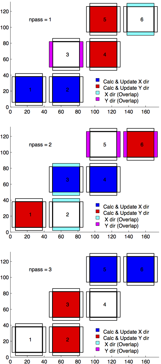
The minimum size of the required tile overlap region (OLx, OLx)
is (stencil size -1)/2. The minimum overlap required by the model in general is 2,
so for some of the above choices the advection scheme will not cost anything in terms of an additional overlap requirement,
but especially given a small tile size, using scheme 7 for example would require costly additional overlap points
(note a cube sphere grid with a “wet-corner” requires doubling this overlap!)
In the ‘Comments’ column, \(\tau\) refers to tracer advection, \(\vec{v}\) momentum advection.
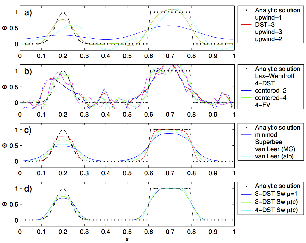
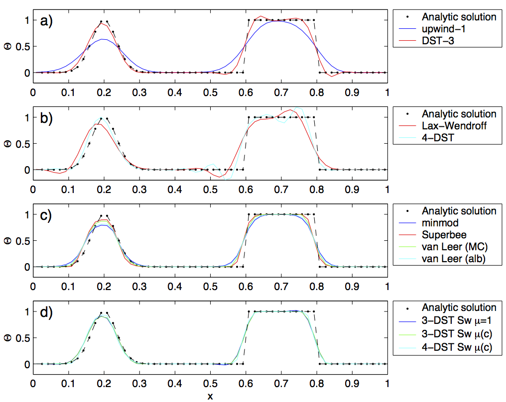
Shown in Figure 2.12 and Figure 2.13 is a 1-D comparison of advection schemes. Here we advect both a smooth hill and a hill with a more abrupt shock.
Figure 2.12 shown the result for a weak flow (low Courant number) whereas Figure 2.13 shows the result for a stronger flow (high Courant number).
Figure 2.12 Comparison of 1-D advection schemes: Courant number is 0.05 with 60 points and solutions are shown for T=1 (one complete period). a) Shows the upwind biased schemes; first order upwind, DST3, third order upwind and second order upwind. b) Shows the centered schemes; Lax-Wendroff, DST4, centered second order, centered fourth order and finite volume fourth order. c) Shows the second order flux limiters: minmod, Superbee, MC limiter and the van Leer limiter. d) Shows the DST3 method with flux limiters due to Sweby with \(\mu =1\) , \(\mu =c/(1-c)\) and a fourth order DST method with Sweby limiter, \(\mu =c/(1-c)\) .
Figure 2.13 Comparison of 1-D advection schemes: Courant number is 0.89 with 60 points and solutions are shown for T=1 (one complete period). a) Shows the upwind biased schemes; first order upwind and DST3. Third order upwind and second order upwind are unstable at this Courant number. b) Shows the centered schemes; Lax-Wendroff, DST4. Centered second order, centered fourth order and finite volume fourth order are unstable at this Courant number. c) Shows the second order flux limiters: minmod, Superbee, MC limiter and the van Leer limiter. d) Shows the DST3 method with flux limiters due to Sweby with \(\mu =1\) , \(\mu =c/(1-c)\) and a fourth order DST method with Sweby limiter, \(\mu =c/(1-c)\) .
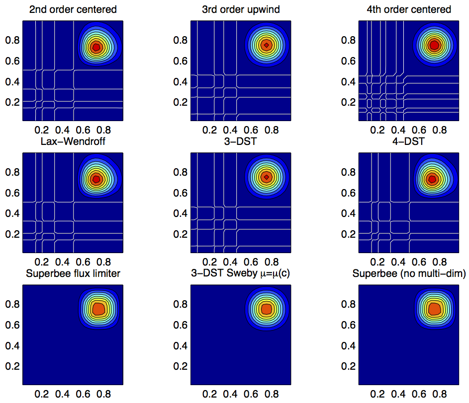
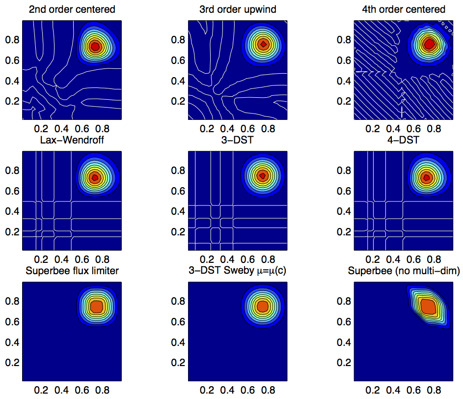
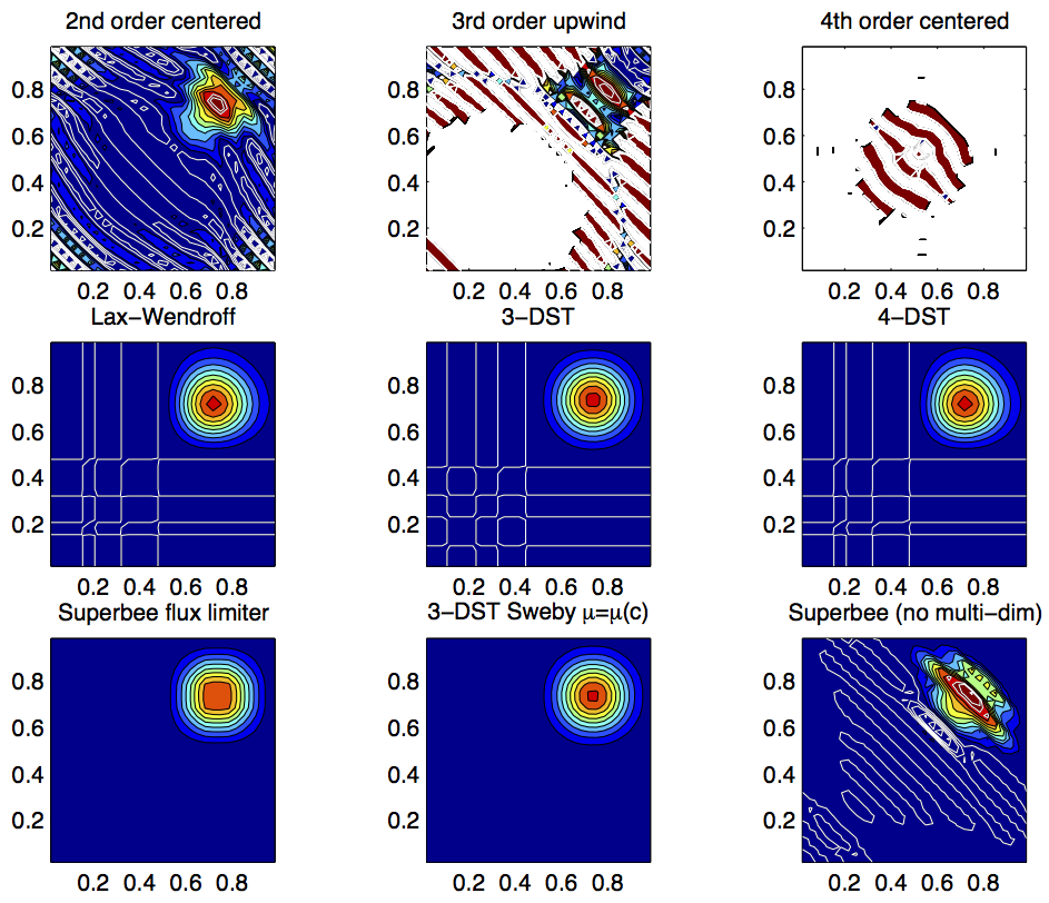
Figure 2.14, Figure 2.15 and
Figure 2.16 show solutions to a simple diagonal advection
problem using a selection of schemes for low, moderate and high Courant
numbers, respectively. The top row shows the linear schemes, integrated
with the Adams-Bashforth method. Theses schemes are clearly unstable for
the high Courant number and weakly unstable for the moderate Courant
number. The presence of false extrema is very apparent for all Courant
numbers. The middle row shows solutions obtained with the unlimited but
multi-dimensional schemes. These solutions also exhibit false extrema
though the pattern now shows symmetry due to the multi-dimensional
scheme. Also, the schemes are stable at high Courant number where the
linear schemes weren’t. The bottom row (left and middle) shows the
limited schemes and most obvious is the absence of false extrema. The
accuracy and stability of the unlimited non-linear schemes is retained
at high Courant number but at low Courant number the tendency is to
lose amplitude in sharp peaks due to diffusion. The one dimensional
tests shown in Figure 2.12 and Figure 2.13 show
this phenomenon.
Finally, the bottom left and right panels use the same advection scheme
but the right does not use the multi-dimensional method. At low Courant
number this appears to not matter but for moderate Courant number severe
distortion of the feature is apparent. Moreover, the stability of the
multi-dimensional scheme is determined by the maximum Courant number
applied of each dimension while the stability of the method of lines is
determined by the sum. Hence, in the high Courant number plot, the
scheme is unstable.
Figure 2.14 Comparison of advection schemes in two dimensions; diagonal advection of a resolved Gaussian feature. Courant number is 0.01 with 30 \(\times\) 30 points and solutions are shown for T=1/2. White lines indicate zero crossing (ie. the presence of false minima). The left column shows the second order schemes; top) centered second order with Adams-Bashforth, middle) Lax-Wendroff and bottom) Superbee flux limited. The middle column shows the third order schemes; top) upwind biased third order with Adams-Bashforth, middle) third order direct space-time method and bottom) the same with flux limiting. The top right panel shows the centered fourth order scheme with Adams-Bashforth and right middle panel shows a fourth order variant on the DST method. Bottom right panel shows the Superbee flux limiter (second order) applied independently in each direction (method of lines).
Figure 2.15 Comparison of advection schemes in two dimensions; diagonal advection of a resolved Gaussian feature. Courant number is 0.27 with 30 \(\times\) 30 points and solutions are shown for T=1/2. White lines indicate zero crossing (ie. the presence of false minima). The left column shows the second order schemes; top) centered second order with Adams-Bashforth, middle) Lax-Wendroff and bottom) Superbee flux limited. The middle column shows the third order schemes; top) upwind biased third order with Adams-Bashforth, middle) third order direct space-time method and bottom) the same with flux limiting. The top right panel shows the centered fourth order scheme with Adams-Bashforth and right middle panel shows a fourth order variant on the DST method. Bottom right panel shows the Superbee flux limiter (second order) applied independently in each direction (method of lines).
Figure 2.16 Comparison of advection schemes in two dimensions; diagonal advection of a resolved Gaussian feature. Courant number is 0.47 with 30 \(\times\) 30 points and solutions are shown for T=1/2. White lines indicate zero crossings and initial maximum values (ie. the presence of false extrema). The left column shows the second order schemes; top) centered second order with Adams-Bashforth, middle) Lax-Wendroff and bottom) Superbee flux limited. The middle column shows the third order schemes; top) upwind biased third order with Adams-Bashforth, middle) third order direct space-time method and bottom) the same with flux limiting. The top right panel shows the centered fourth order scheme with Adams-Bashforth and right middle panel shows a fourth order variant on the DST method. Bottom right panel shows the Superbee flux limiter (second order) applied independently in each direction (method of lines).
With many advection schemes implemented in the code two questions arise:
“Which scheme is best?” and “Why don’t you just offer the best advection
scheme?”. Unfortunately, no one advection scheme is “the best” for all
particular applications and for new applications it is often a matter of
trial to determine which is most suitable. Here are some guidelines but
these are not the rule;
If you have a coarsely resolved model, using a positive or upwind
biased scheme will introduce significant diffusion to the solution
and using a centered higher order scheme will introduce more noise.
In this case, simplest may be best.
If you have a high resolution model, using a higher order scheme will
give a more accurate solution but scale-selective diffusion might
need to be employed. The flux limited methods offer similar accuracy
in this regime.
If your solution has shocks or propagating fronts then a flux limited
scheme is almost essential.
If your time-step is limited by advection, the multi-dimensional
non-linear schemes have the most stability (up to Courant number 1).
If you need to know how much diffusion/dissipation has occurred you
will have a lot of trouble figuring it out with a non-linear method.
The presence of false extrema is non-physical and this alone is the
strongest argument for using a positive scheme.