This document provides the reader with the information necessary to
carry out numerical experiments using MITgcm. It gives a comprehensive
description of the continuous equations on which the model is based, the
numerical algorithms the model employs and a description of the associated
program code. Along with the hydrodynamical kernel, physical and
biogeochemical parameterizations of key atmospheric and oceanic processes
are available. A number of examples illustrating the use of the model in
both process and general circulation studies of the atmosphere and ocean are
also presented.
it can be used to study both atmospheric and oceanic phenomena; one hydrodynamical kernel is used to drive forward both atmospheric and oceanic models - see Figure 1.1
Figure 1.1 MITgcm has a single dynamical kernel that can drive forward either oceanic or atmospheric simulations.
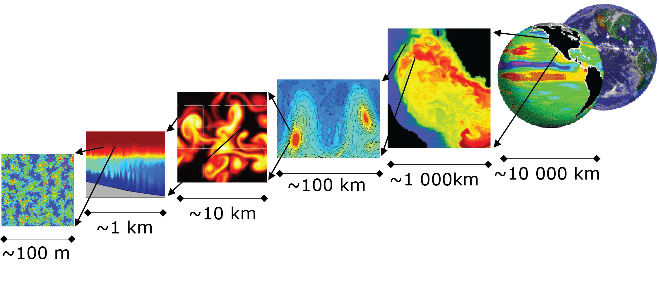
it has a non-hydrostatic capability and so can be used to study both small-scale and large scale processes - see Figure 1.2
Figure 1.2 MITgcm has non-hydrostatic capabilities, allowing the model to address a wide range of phenomenon - from convection on the left, all the way through to global circulation patterns on the right.
finite volume techniques are employed yielding an intuitive discretization and support for the treatment of irregular geometries using orthogonal curvilinear grids and shaved cells - see Figure 1.3
Figure 1.3 Finite volume techniques (bottom panel) are used, permitting a treatment of topography that rivals \(\sigma\) (terrain following) coordinates.
tangent linear and adjoint counterparts are automatically maintained along with the forward model, permitting sensitivity and optimization studies.
the model is developed to perform efficiently on a wide variety of computational platforms.
Key publications reporting on and charting the development of the model are Hill and Marshall (1995), Marshall et al. (1997a),
Marshall et al. (1997b), Adcroft and Marshall (1997), Marshall et al. (1998), Adcroft and Marshall (1999), Hill et al. (1999),
Marotzke et al. (1999), Adcroft and Campin (2004), Adcroft et al. (2004b), Marshall et al. (2004) (an overview on the model formulation can also be found in Adcroft et al. (2004c)):
Hill, C. and J. Marshall, (1995)
Application of a Parallel Navier-Stokes Model to Ocean Circulation in
Parallel Computational Fluid Dynamics,
In Proceedings of Parallel Computational Fluid Dynamics: Implementations
and Results Using Parallel Computers, 545-552.
Elsevier Science B.V.: New York [HM95]
Marshall, J., C. Hill, L. Perelman, and A. Adcroft, (1997a)
Hydrostatic, quasi-hydrostatic, and nonhydrostatic ocean modeling,
J. Geophysical Res., 102(C3), 5733-5752 [MHPA97]
Marshall, J., A. Adcroft, C. Hill, L. Perelman, and C. Heisey, (1997b)
A finite-volume, incompressible Navier Stokes model for studies of the ocean
on parallel computers, J. Geophysical Res., 102(C3), 5753-5766 [MAH+97]
Adcroft, A.J., Hill, C.N. and J. Marshall, (1997)
Representation of topography by shaved cells in a height coordinate ocean
model, Mon Wea Rev, 125, 2293-2315 [AHM97]
Marshall, J., Jones, H. and C. Hill, (1998)
Efficient ocean modeling using non-hydrostatic algorithms,
Journal of Marine Systems, 18, 115-134 [MJH98]
Adcroft, A., Hill C. and J. Marshall: (1999)
A new treatment of the Coriolis terms in C-grid models at both high and low
resolutions,
Mon. Wea. Rev., 127, 1928-1936 [AHM99]
Hill, C, Adcroft,A., Jamous,D., and J. Marshall, (1999)
A Strategy for Terascale Climate Modeling,
In Proceedings of the Eighth ECMWF Workshop on the Use of Parallel Processors
in Meteorology, 406-425
World Scientific Publishing Co: UK [HAJM99]
Marotzke, J, Giering,R., Zhang, K.Q., Stammer,D., Hill,C., and T.Lee, (1999)
Construction of the adjoint MIT ocean general circulation model and
application to Atlantic heat transport variability,
J. Geophysical Res., 104(C12), 29,529-29,547 [MGZ+99]
A. Adcroft and J.-M. Campin, (2004a)
Re-scaled height coordinates for accurate representation of free-surface flows in ocean circulation models,
Ocean Modelling, 7, 269–284 [AC04]
A. Adcroft, J.-M. Campin, C. Hill, and J. Marshall, (2004b)
Implementation of an atmosphere-ocean general circulation model on the expanded
spherical cube,
Mon Wea Rev , 132, 2845–2863 [ACHM04]
J. Marshall, A. Adcroft, J.-M. Campin, C. Hill, and A. White, (2004)
Atmosphere-ocean modeling exploiting fluid isomorphisms, Mon. Wea. Rev., 132, 2882–2894 [MAC+04]
A. Adcroft, C. Hill, J.-M. Campin, J. Marshall, and P. Heimbach, (2004c)
Overview of the formulation and numerics of the MITgcm, In Proceedings of the ECMWF seminar series on Numerical Methods, Recent developments in numerical methods for atmosphere and ocean modelling, 139–149. URL: http://mitgcm.org/pdfs/ECMWF2004-Adcroft.pdf[AHJMC+04]
We begin by briefly showing some of the results of the model in action to
give a feel for the wide range of problems that can be addressed using it.
MITgcm has been designed and used to model a wide range of phenomena,
from convection on the scale of meters in the ocean to the global pattern of
atmospheric winds - see Figure 1.2. To give a flavor of the
kinds of problems the model has been used to study, we briefly describe some
of them here. A more detailed description of the underlying formulation,
numerical algorithm and implementation that lie behind these calculations is
given later. Indeed many of the illustrative examples shown below can be
easily reproduced: simply download the model (the minimum you need is a PC
running Linux, together with a FORTRAN77 compiler) and follow the examples
described in detail in the documentation.
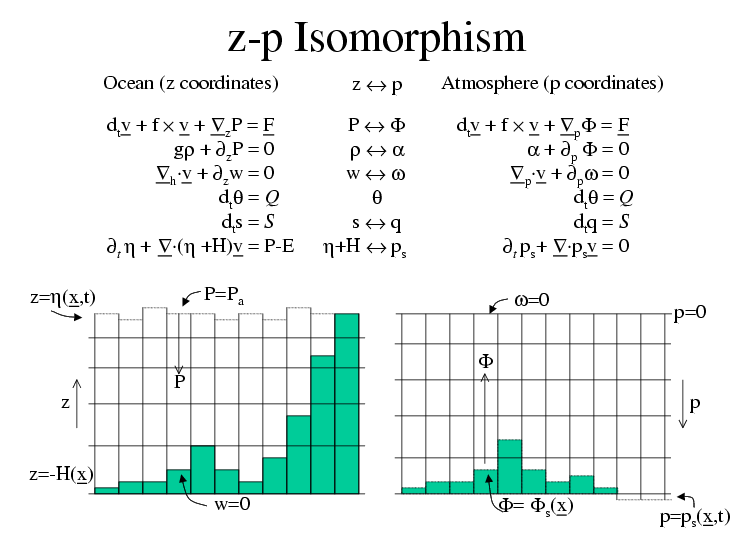
To render atmosphere and ocean models from one dynamical core we exploit
‘isomorphisms’ between equation sets that govern the evolution of the
respective fluids - see Figure 1.17. One system of
hydrodynamical equations is written down and encoded. The model
variables have different interpretations depending on whether the
atmosphere or ocean is being studied. Thus, for example, the vertical
coordinate ‘\(r\)’ is interpreted as pressure, \(p\), if we are
modeling the atmosphere (right hand side of Figure 1.17) and height, \(z\), if we are modeling
the ocean (left hand side of Figure 1.17).
Figure 1.17 Isomorphic equation sets used for atmosphere (right) and ocean (left).
The state of the fluid at any time is characterized by the distribution
of velocity \(\vec{\mathbf{v}}\), active tracers \(\theta\) and
\(S\), a ‘geopotential’ \(\phi\) and density
\(\rho =\rho (\theta ,S,p)\) which may depend on \(\theta\),
\(S\), and \(p\). The equations that govern the evolution of
these fields, obtained by applying the laws of classical mechanics and
thermodynamics to a Boussinesq, Navier-Stokes fluid are, written in
terms of a generic vertical coordinate, \(r\), so that the
appropriate kinematic boundary conditions can be applied isomorphically
see Figure 1.18.
Figure 1.18 Vertical coordinates and kinematic boundary conditions for atmosphere (top) and ocean (bottom).
\[\frac{D}{Dt}=\frac{\partial }{\partial t}+\vec{\mathbf{v}}\cdot \nabla \text{ is the total derivative}\]
\[ \nabla = \nabla _{h}+\hat{\boldsymbol{k}}\frac{\partial }{\partial r}
\text{ is the ‘grad’ operator}\]
with \(\nabla _{h}\) operating in the horizontal and
\(\hat{\boldsymbol{k}}
\frac{\partial }{\partial r}\) operating in the vertical, where
\(\hat{\boldsymbol{k}}\) is a unit vector in the vertical
\[t\text{ is time}\]
\[\vec{\mathbf{v}}=(u,v,\dot{r})=(\vec{\mathbf{v}}_{h},\dot{r})\text{ is the velocity}\]
\[\phi \text{ is the ‘pressure’/‘geopotential’}\]
\[\vec{\boldsymbol{\Omega}}\text{ is the Earth's rotation}\]
\[b\text{ is the ‘buoyancy’}\]
\[\theta \text{ is potential temperature}\]
\[S\text{ is specific humidity in the atmosphere; salinity in the ocean}\]
\[\vec{\boldsymbol{\mathcal{F}}}\text{ are forcing and dissipation of }\vec{
\mathbf{v}}\]
\[\mathcal{Q}_{\theta }\mathcal{\ }\text{ are forcing and dissipation of }\theta\]
\[\mathcal{Q}_{S}\mathcal{\ }\text{are forcing and dissipation of }S\]
The terms \(\vec{\boldsymbol{\mathcal{F}}}\) and \(\mathcal{Q}\)
are provided by ‘physics’ and forcing packages for atmosphere and ocean.
These are described in later chapters.