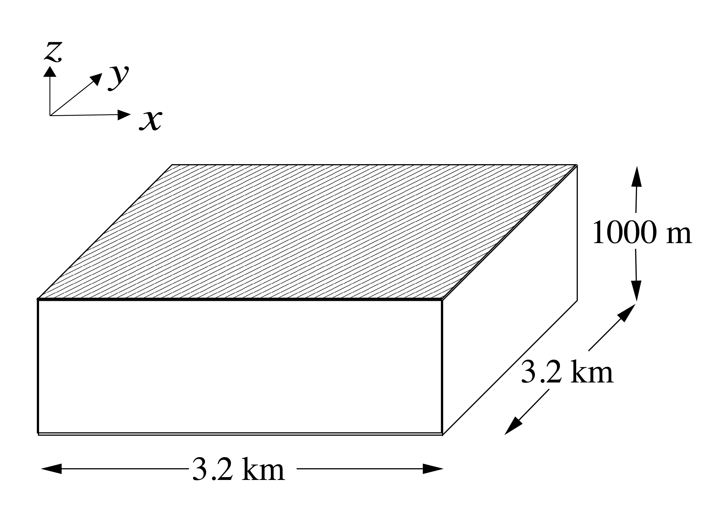
Figure 4.39 Schematic of simulation domain for the surface driven convection experiment. The domain is doubly periodic with an initially uniform temperature of 20 oC.
This experiment, Figure 4.39, showcasing
MITgcm’s non-hydrostatic capability, was designed to explore the
temporal and spatial characteristics of convection plumes as they might
exist during a period of oceanic deep convection. It is
The model domain consists of an approximately 3 km square by 1 km deep
box of initially unstratified, resting fluid. The domain is doubly
periodic.
The experiment has 20 levels in the vertical, each of equal thickness
\(\Delta z =\) 50 m (the horizontal resolution is also 50 m). The
fluid is initially unstratified with a uniform reference potential
temperature \(\theta =\) 20 oC. The equation of state
used in this experiment is linear
with \(\rho_{0}=1000\,{\rm kg\,m}^{-3}\) and
\(\alpha_{\theta}=2\times10^{-4}\,{\rm degrees}^{-1}\). Integrated
forward in this configuration, the model state variable theta is
equivalent to either in-situ temperature, \(T\), or potential
temperature, \(\theta\). For consistency with other examples, in
which the equation of state is non-linear, we use \(\theta\) to
represent temperature here. This is the quantity that is carried in the
model core equations.
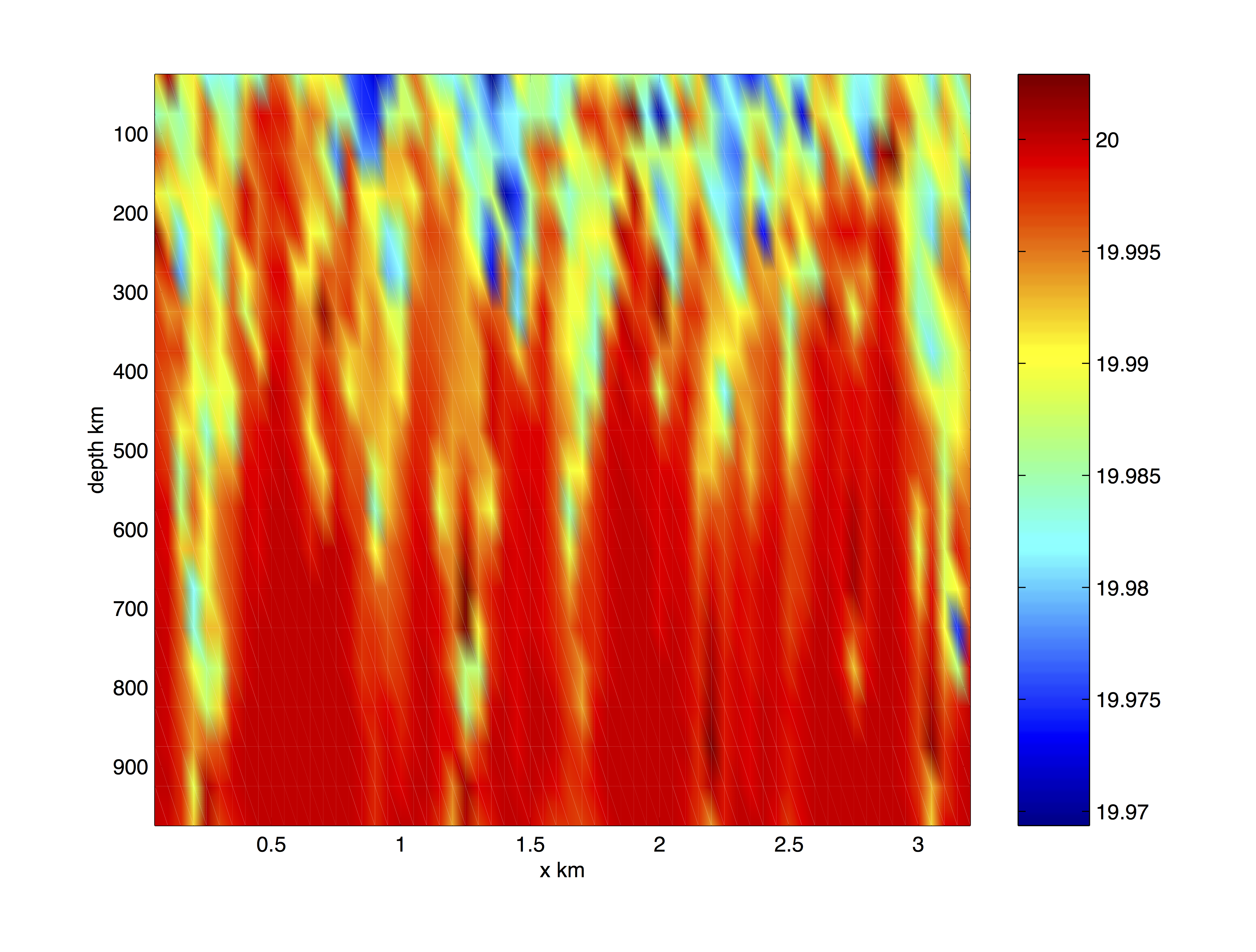
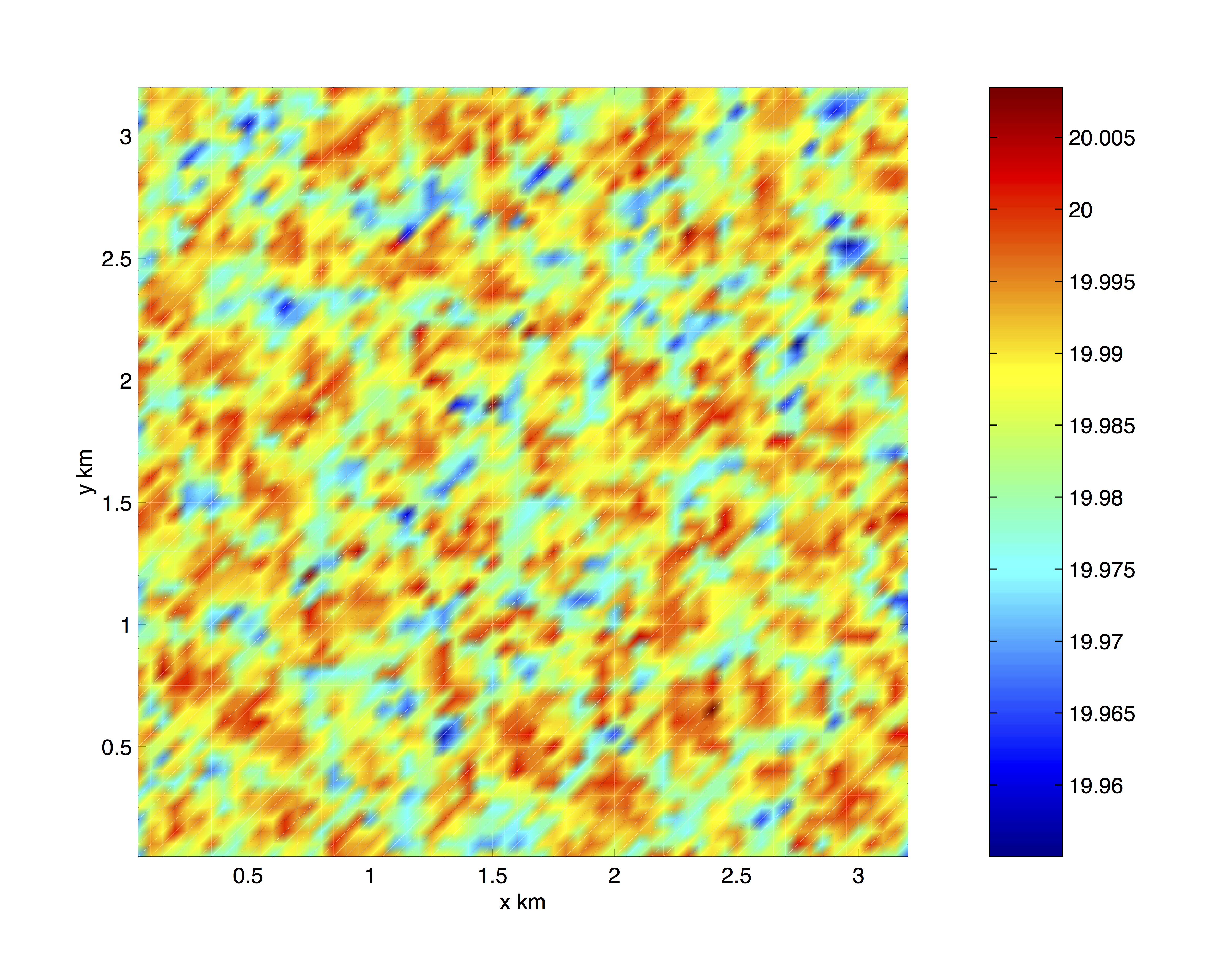
As the fluid in the surface layer is cooled (at a mean rate of 800
Wm\(^2\)), it becomes convectively unstable and overturns, at
first close to the grid-scale, but, as the flow matures, on larger
scales (Figure 4.40 and
Figure 4.41), under the influence of rotation
(\(f_o = 10^{-4}\) s\(^{-1}\)).
Model parameters are specified in file input/data. The grid dimensions
are prescribed in code/SIZE.h. The forcing (file input/Qsurf.bin) is
specified in a binary data file generated using the Matlab script
input/gendata.m.
The model is configured in non-hydrostatic form, that is, all terms in
the Navier Stokes equations are retained and the pressure field is
found, subject to appropriate boundary conditions, through inversion of
a 3-D elliptic equation.
The implicit free surface form of the pressure equation described in
Marshall et. al (1997) [MHPA97] is employed. A
horizontal Laplacian operator \(\nabla_{h}^2\) provides viscous
dissipation. The thermodynamic forcing appears as a sink in the
equation for potential temperature \(\theta\). This produces a set of equations
solved in this configuration as follows:
where \(u=\frac{Dx}{Dt}\), \(v=\frac{Dy}{Dt}\) and
\(w=\frac{Dz}{Dt}\) are the components of the flow vector in
directions \(x\), \(y\) and \(z\). The pressure is
diagnosed through inversion (subject to appropriate boundary
conditions) of a 3-D elliptic equation derived from the divergence of
the momentum equations and continuity (see Section 1.3.6).
The domain is discretized with a uniform grid spacing in each direction.
There are 64 grid cells in directions \(x\) and \(y\) and 20
vertical levels thus the domain comprises a total of just over 80,000
gridpoints.
4.8.4. Numerical stability criteria and other considerations
For a heat flux of 800 Wm\(^2\) and a rotation rate of
\(10^{-4}\) s\(^{-1}\) the plume-scale can be expected to be a
few hundred meters guiding our choice of grid resolution. This in turn
restricts the timestep we can take. It is also desirable to minimize the
level of diffusion and viscosity we apply.
For this class of problem it is generally the advective time-scale which
restricts the timestep.
For an extreme maximum flow speed of \(| \vec{u} | = 1 ms^{-1}\),
at a resolution of 50 m, the implied maximum timestep for stability,
\(\delta t_u\) is
The choice of \(\delta t = 10\) s is a safe 20 percent of this
maximum.
Interpreted in terms of a mixing-length hypothesis, a magnitude of
Laplacian diffusion coefficient \(\kappa_h (=
\kappa_v) = 0.1\) m\(^2\)s\(^{-1}\) is consistent with an
eddy velocity of 2 mm s\(^{-1}\) correlated over 50 m.
1CBOP
2C !ROUTINE: SIZE.h
3C !INTERFACE:
4C include SIZE.h
5C !DESCRIPTION: \bv
6C *==========================================================*
7C | SIZE.h Declare size of underlying computational grid.
8C *==========================================================*
9C | The design here supports a three-dimensional model grid
10C | with indices I,J and K. The three-dimensional domain
11C | is comprised of nPx*nSx blocks (or tiles) of size sNx
12C | along the first (left-most index) axis, nPy*nSy blocks
13C | of size sNy along the second axis and one block of size
14C | Nr along the vertical (third) axis.
15C | Blocks/tiles have overlap regions of size OLx and OLy
16C | along the dimensions that are subdivided.
17C *==========================================================*
18C \ev
19C
20C Voodoo numbers controlling data layout:
21C sNx :: Number of X points in tile.
22C sNy :: Number of Y points in tile.
23C OLx :: Tile overlap extent in X.
24C OLy :: Tile overlap extent in Y.
25C nSx :: Number of tiles per process in X.
26C nSy :: Number of tiles per process in Y.
27C nPx :: Number of processes to use in X.
28C nPy :: Number of processes to use in Y.
29C Nx :: Number of points in X for the full domain.
30C Ny :: Number of points in Y for the full domain.
31C Nr :: Number of points in vertical direction.
32CEOP
33 INTEGER sNx
34 INTEGER sNy
35 INTEGER OLx
36 INTEGER OLy
37 INTEGER nSx
38 INTEGER nSy
39 INTEGER nPx
40 INTEGER nPy
41 INTEGER Nx
42 INTEGER Ny
43 INTEGER Nr
44 PARAMETER (
45 & sNx = 50,
46 & sNy = 50,
47 & OLx = 2,
48 & OLy = 2,
49 & nSx = 2,
50 & nSy = 2,
51 & nPx = 1,
52 & nPy = 1,
53 & Nx = sNx*nSx*nPx,
54 & Ny = sNy*nSy*nPy,
55 & Nr = 50)
5657C MAX_OLX :: Set to the maximum overlap region size of any array
58C MAX_OLY that will be exchanged. Controls the sizing of exch
59C routine buffers.
60 INTEGER MAX_OLX
61 INTEGER MAX_OLY
62 PARAMETER ( MAX_OLX = OLx,
63 & MAX_OLY = OLy )
64
Three lines are customized in this file. These prescribe the domain grid
dimensions.
Line 45,
sNx=50,
this line sets the lateral domain extent in grid points for the axis
aligned with the \(x\)-coordinate.
Line 46,
sNy=50,
this line sets the lateral domain extent in grid points for the axis
aligned with the \(y\)-coordinate.
Line 55,
Nr=50,
this line sets the vertical domain extent in grid points.
This file specifies the main parameters
for the experiment. The parameters that are significant for this
configuration are
Line 7,
tRef=20*20.0,
this line sets the initial and reference values of potential
temperature at each model level in units of
\(^{\circ}\mathrm{C}\). Here the value is arbitrary since, in
this case, the flow evolves independently of the absolute magnitude
of the reference temperature. For each depth level the initial and
reference profiles will be uniform in \(x\) and \(y\).
Line 8,
sRef=20*35.0,
this line sets the initial and reference values of salinity at each
model level in units of ppt. In this case salinity is set to an
(arbitrary) uniform value of 35.0 ppt. However since, in this
example, density is independent of salinity, an appropriately defined
initial salinity could provide a useful passive tracer. For each
depth level the initial and reference profiles will be uniform in
\(x\) and \(y\).
Line 9,
viscAh=0.1,
this line sets the horizontal Laplacian dissipation coefficient to
0.1 \({\rm m^{2}s^{-1}}\). Boundary conditions for this operator
are specified later.
Line 10,
viscAz=0.1,
this line sets the vertical Laplacian frictional dissipation
coefficient to 0.1 \({\rm m^{2}s^{-1}}\). Boundary conditions for
this operator are specified later.
Line 11,
no_slip_sides=.FALSE.
this line selects a free-slip lateral boundary condition for the
horizontal Laplacian friction operator e.g.
\(\frac{\partial u}{\partial y}\)=0 along boundaries in
\(y\) and \(\frac{\partial v}{\partial x}\)=0 along
boundaries in \(x\).
Lines 12,
no_slip_bottom=.TRUE.
this line selects a no-slip boundary condition for the bottom
boundary condition in the vertical Laplacian friction operator e.g.,
\(u=v=0\) at \(z=-H\), where \(H\) is the local depth of
the domain.
Line 13,
diffKhT=0.1,
this line sets the horizontal diffusion coefficient for temperature
to 0.1 \(\rm m^{2}s^{-1}\). The boundary condition on this
operator is
\(\frac{\partial}{\partial x}=\frac{\partial}{\partial y}=0\) at
all boundaries.
Line 14,
diffKzT=0.1,
this line sets the vertical diffusion coefficient for temperature to
0.1 \({\rm m^{2}s^{-1}}\). The boundary condition on this
operator is \(\frac{\partial}{\partial z}\) = 0 on all
boundaries.
Line 15,
f0=1E-4,
this line sets the Coriolis parameter to \(1 \times 10^{-4}\)
s\(^{-1}\). Since \(\beta = 0.0\) this value is then
adopted throughout the domain.
Line 16,
beta=0.E-11,
this line sets the the variation of Coriolis parameter with latitude
to \(0\).
Line 17,
tAlpha=2.E-4,
This line sets the thermal expansion coefficient for the fluid to
\(2 \times 10^{-4}\)oC\(^{-1}\).
Line 18,
sBeta=0,
This line sets the saline expansion coefficient for the fluid to
\(0\), consistent with salt’s passive role in this example.
Line 23-24,
rigidLid=.FALSE.,
implicitFreeSurface=.TRUE.,
Selects the barotropic pressure equation to be the implicit free
surface formulation.
Line 26,
eosType='LINEAR',
Selects the linear form of the equation of state.
Line 27,
nonHydrostatic=.TRUE.,
Selects for non-hydrostatic code.
Line 33,
cg2dMaxIters=1000,
Inactive - the pressure field in a non-hydrostatic simulation is
inverted through a 3-D elliptic equation.
Line 34,
cg2dTargetResidual=1.E-9,
Inactive - the pressure field in a non-hydrostatic simulation is
inverted through a 3-D elliptic equation.
Line 35,
cg3dMaxIters=40,
This line sets the maximum number of iterations the
3-D conjugate gradient solver will use to 40,
irrespective of the convergence criteria being met.
Line 36,
cg3dTargetResidual=1.E-9,
Sets the tolerance which the 3-D conjugate gradient
solver will use to test for convergence in equation (2.61) to
\(1 \times 10^{-9}\). The solver will iterate until the tolerance
falls below this value or until the maximum number of solver
iterations is reached.
Line43,
nTimeSteps=8640.,
Sets the number of timesteps at which this simulation will terminate
(in this case 8640 timesteps or 1 day or \(\delta t = 10\) s). At
the end of a simulation a checkpoint file is automatically written so
that a numerical experiment can consist of multiple stages.
Line 44,
deltaT=10,
Sets the timestep \(\delta t\) to 10 s.
Line 57,
dXspacing=50.0,
Sets horizontal (\(x\)-direction) grid interval to 50 m.
Line 58,
dYspacing=50.0,
Sets horizontal (\(y\)-direction) grid interval to 50 m.
Line 59,
delZ=20*50.0,
Sets vertical grid spacing to 50 m. Must be consistent with
code/SIZE.h.
Here, 20 corresponds to the number of vertical levels.
Line64,
surfQfile='Qsurf.bin'
This line specifies the name of the file from which the surface heat
flux is read. This file is a 2-D (\(x,y\)) map. It is
assumed to contain 64-bit binary numbers giving the value of
\(Q\) (W m\(^2\)) to be applied in each surface grid cell,
ordered with the \(x\) coordinate varying fastest. The points are
ordered from low coordinate to high coordinate for both axes. The
matlab program input/gendata.m
shows how to generate the surface
heat flux file used in the example.
The file input/Qsurf.bin specifies a 2-D (\(x,y\)) map
of heat flux values where
\(Q = Q_o \times ( 0.5 + \mbox{random number between 0 and 1})\).
In the example \(Q_o = 800\) W m\(^{-2}\) so that values of
\(Q\) lie in the range 400 to 1200 W m\(^{-2}\) with a mean of
\(Q_o\). Although the flux models a loss, because it is directed
upwards, according to the model’s sign convention, \(Q\) is
positive.