4.4. Ocean Gyre Advection Schemes
(in directory: verification/tutorial_advection_in_gyre/)
This set of examples is based on the barotropic and baroclinic gyre MITgcm configurations, that are described in Section 4.1 and Section 4.2. The examples in this section explain how to introduce a passive tracer into the flow field of the barotropic and baroclinic gyre setups and looks at how the time evolution of the passive tracer depends on the advection or transport scheme that is selected for the tracer.
Passive tracers are useful in many numerical experiments. In some cases tracers are used to track flow pathways, for example in Dutay et al. (2002) [DBD+02] a passive tracer is used to track pathways of CFC-11 in 13 global ocean models, using a numerical configuration similar to the example described in Section 4.13). In other cases tracers are used as a way to infer bulk mixing coefficients for a turbulent flow field, for example in Marshall et al. (2006) [MSJH06] a tracer is used to infer eddy mixing coefficients in the Antarctic Circumpolar Current region. Typically, in biogeochemical and ecological simulations large numbers of tracers are used that carry the concentrations of biological nutrients and concentrations of biological species. When using tracers for these and other purposes it is useful to have a feel for the role that the advection scheme employed plays in determining properties of the tracer distribution. In particular, in a discrete numerical model, tracer advection only approximates the continuum behavior in space and time and different advection schemes introduce different approximations so that the resulting tracer distributions vary. In the following text we illustrate how to use the different advection schemes available in MITgcm, and discuss which properties are well represented by each scheme. The advection schemes selections also apply to active tracers (e.g., \(T\) and \(S\)) and the character of the schemes also affects their distributions and behavior.
4.4.1. Advection and tracer transport
In general, the tracer problem we want to solve can be written
where \(C\) is the tracer concentration in a model cell, \(\vec{\bf U}=(u,v,w)\) is the model 3-D flow field. In (4.29), \(S\) represents source, sink and tendency terms not associated with advective transport. Example of terms in \(S\) include (i) air-sea fluxes for a dissolved gas, (ii) biological grazing and growth terms (for a biogeochemical problem) or (iii) convective mixing and other sub-grid parameterizations of mixing. In this section we are primarily concerned with
how to introduce the tracer term, \(C\), into an integration
the different discretized forms of the \(-\vec{\bf U} \cdot \nabla C\) term that are available
4.4.2. Introducing a tracer into the flow
The MITgcm ptracers package (see section Section 8.3.3 for a more complete discussion of the ptracers package and section Section 8.1.1 for a general introduction to MITgcm packages) provides pre-coded support for a simple passive tracer with an initial distribution at simulation time \(t=0\) of \(C_0(x,y,z)\). The steps required to use this capability are
Activating the ptracers package. This simply requires adding the line
ptracersto the file code/packages.conf.Setting an initial tracer distribution.
Once the two steps above are complete we can proceed to examine how the tracer we have created is carried by the flow field and what properties of the tracer distribution are preserved under different advection schemes.
4.4.3. Selecting an advection scheme
flags in input/data and input/data.ptracers
overlap width
#defineCPP option PTRACERS_ALLOW_DYN_STATE in code/PTRACERS_OPTIONS.h as required for SOM case
4.4.4. Comparison of different advection schemes
Conservation
Dispersion
Diffusion
Positive definite
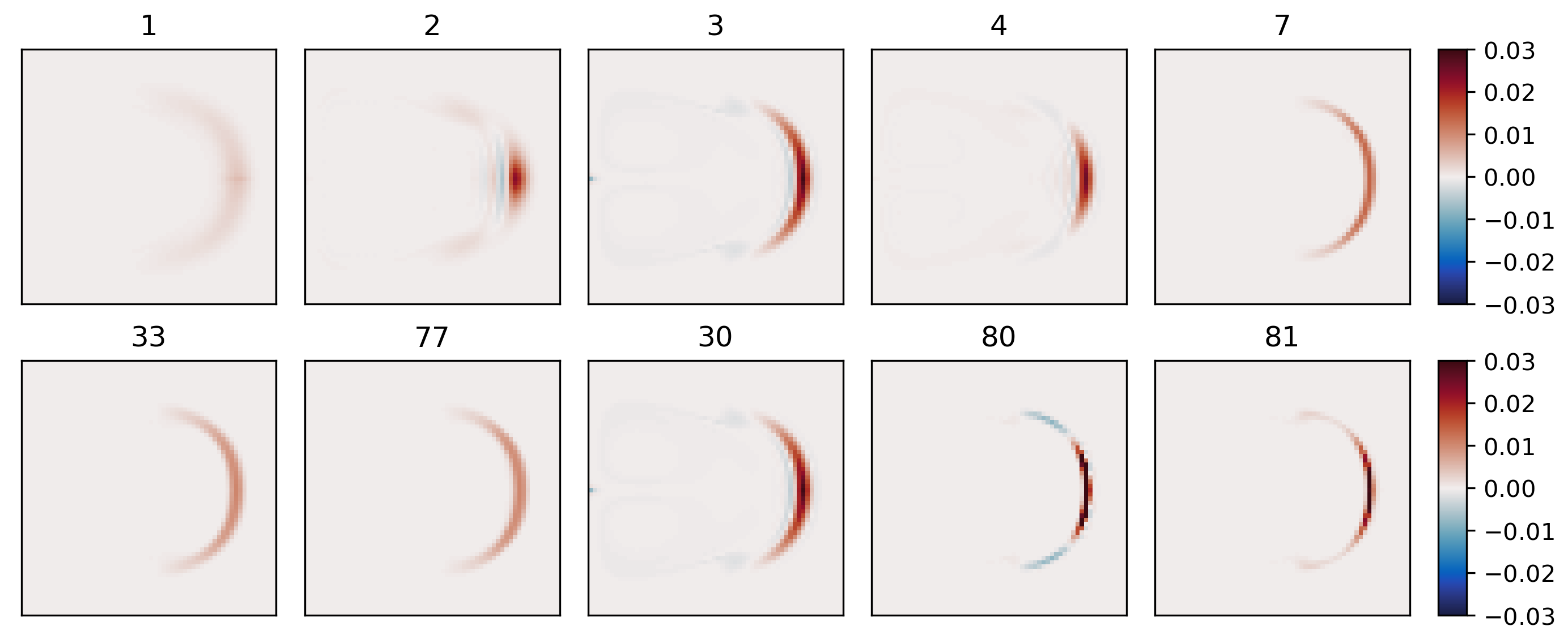
Figure 4.24 Dye evolving in a double gyre with different advection schemes. The figure shows the dye concentration one year after injection into a single grid cell near the left boundary.
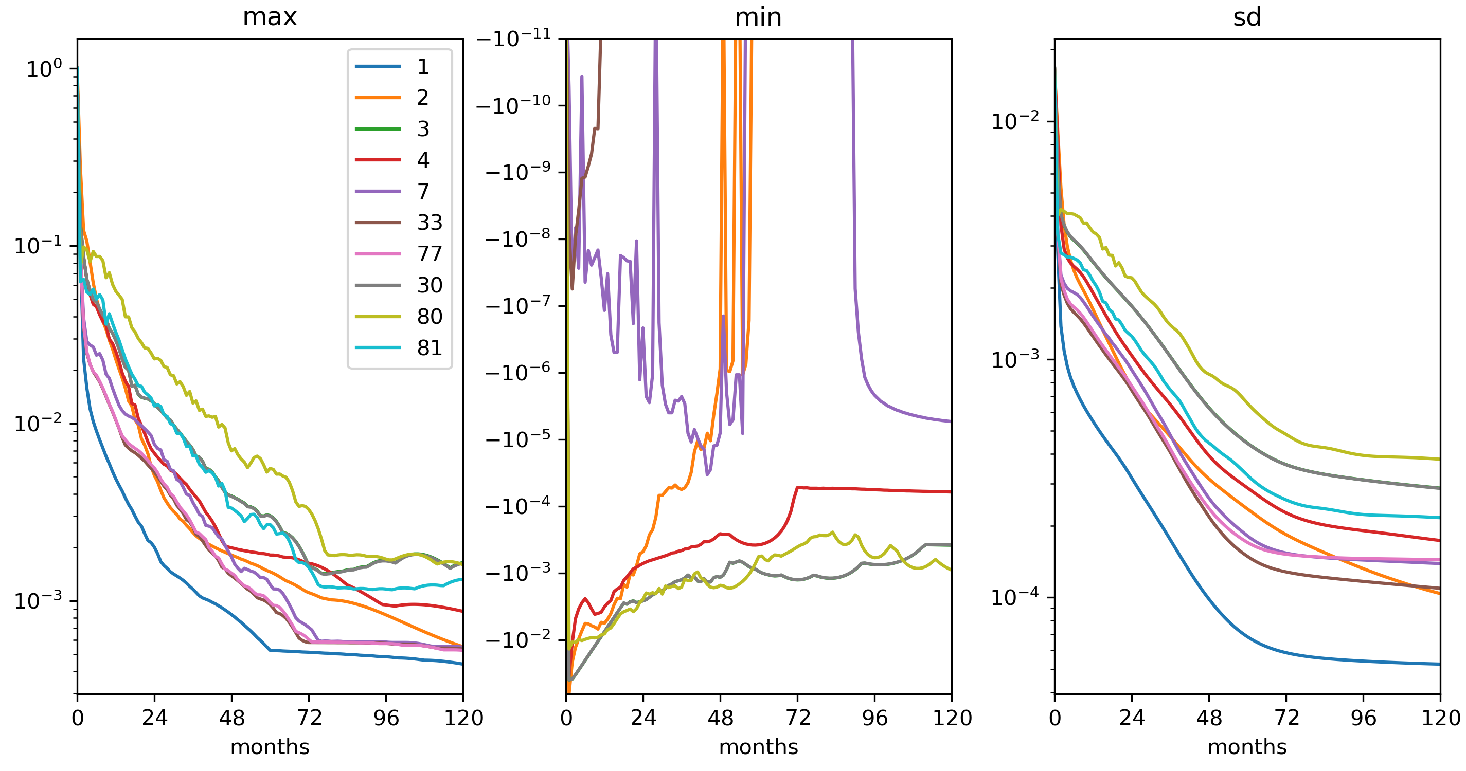
Figure 4.25 Maxima, minima and standard deviation (from left) as a function of time (in months) for the gyre circulation experiment from Figure 4.24.