This example experiment demonstrates using MITgcm to simulate the
planetary ocean circulation in pressure coordinates, that is, without
making the Boussinesq approximations. The simulation is configured as a near
copy of tutorial_global_oce_latlon
(Section 4.5). with realistic geography and
bathymetry on a \(4^{\circ} \times
4^{\circ}\) spherical polar grid. Fifteen levels are used in the
vertical, ranging in thickness from
50.4089 dbar \(\approx\) 50 m at the surface to
710.33 dbar \(\approx\) 690 m at depth, giving a
maximum model depth of
5302.3122 dbar \(\approx\) 5200 m. At this
resolution, the configuration can be integrated forward for thousands of
years on a single processor desktop computer.
The model is forced with climatological wind stress data from
Trenberth (1990) [TOL90] and surface flux data from Jiang et al. (1999)
[JSMR99]. Climatological data (Levitus and Boyer 1994a,b [LB94a, LB94b])
is used to initialize the model
hydrography. Levitus and Boyer seasonal climatology
data is also used throughout the calculation to provide additional
air-sea fluxes. These fluxes are combined with the Jiang et al. climatological
estimates of surface heat flux, resulting in a mixed boundary condition
of the style described in Haney (1971) [Han71]. Altogether, this
yields the following forcing applied in the model surface layer.
where \({\cal F}_{u}\), \({\cal F}_{v}\),
\({\cal F}_{\theta}\), \({\cal F}_{s}\) are the forcing terms in
the zonal and meridional momentum and in the potential temperature and
salinity equations respectively. The term \(\Delta p_{s}\)
represents the top ocean layer thickness in Pa. It is used in
conjunction with a reference density, \(\rho_{FW}\) (here set to
999.8 kg m-3), the surface salinity, \(S\), and a
specific heat capacity, \(C_{p}\) (here set to
4000 J kg-1 K-1), to convert
input dataset values into time tendencies of potential temperature (with
units of oC s-1), salinity (with units
ppt s-1) and velocity (with units m s-2).
The externally supplied forcing fields used in this experiment are
\(\tau_{x}\), \(\tau_{y}\), \(\theta^{\ast}\),
\(\cal{Q}\) and \(\cal{E}-\cal{P}-\cal{R}\). The wind stress
fields (\(\tau_x\), \(\tau_y\)) have units of
N m-2. The temperature forcing fields
(\(\theta^{\ast}\) and \(Q\)) have units of
oC and W m-2 respectively.
The salinity forcing fields (\(\cal{E}-\cal{P}-\cal{R}\)) has units of
m s-1 respectively. The source files and
procedures for ingesting these data into the simulation are described in
the experiment configuration discussion in section
Section 4.5.3.
Due to the pressure coordinate, the model can only be hydrostatic (de Szoeke and Samelson 2002
[dSS02]). The domain is discretized with a uniform
grid spacing in latitude and longitude on the sphere
\(\Delta \phi=\Delta
\lambda=4^{\circ}\), so that there are 90 grid cells in the zonal and
40 in the meridional direction. The internal model coordinate
variables \(x\) and \(y\) are initialized according to
\[\begin{split}\begin{aligned}
x=r\cos(\phi),~\Delta x & = r\cos(\Delta \phi) \\
y=r\lambda,~\Delta y & = r\Delta \lambda \end{aligned}\end{split}\]
Arctic polar regions are not included in this experiment. Meridionally
the model extends from 80oS to
80oN. Vertically the model is configured with
fifteen layers with the following thicknesses
\(\Delta p_{1}\) = 7103300.720021 Pa
\(\Delta p_{2}\) = 6570548.440790 Pa
\(\Delta p_{3}\) = 6041670.010249 Pa
\(\Delta p_{4}\) = 5516436.666057 Pa
\(\Delta p_{5}\) = 4994602.034410 Pa
\(\Delta p_{6}\) = 4475903.435290 Pa
\(\Delta p_{7}\) = 3960063.245801 Pa
\(\Delta p_{8}\) = 3446790.312651 Pa
\(\Delta p_{9}\) = 2935781.405664 Pa
\(\Delta p_{10}\) = 2426722.705046 Pa
\(\Delta p_{11}\) = 1919291.315988 Pa
\(\Delta p_{12}\) = 1413156.804970 Pa
\(\Delta p_{13}\) = 1008846.750166 Pa
\(\Delta p_{14}\) = 705919.025481 Pa
\(\Delta p_{15}\) = 504089.693499 Pa
(here the numeric subscript indicates the model level index number,
\({\tt k}\); note that the surface layer has the highest index
number 15) to give a total depth, \(H\), of -5200 m. In
pressure, this is \(p_{b}^{0}\) = 53023122.566084 Pa. The
implicit free surface form of the pressure equation described in
Marshall et al. (1997) [MHPA97] with the nonlinear extension by Campin et al. (2004)
[CAHM04] is employed. A Laplacian operator,
\(\nabla^2\), provides viscous dissipation. Thermal and haline
diffusion is also represented by a Laplacian operator.
Wind-stress forcing is added to the momentum equations in
(4.46) for both the
zonal flow, \(u\) and the meridional flow \(v\), according to
equations (4.42) and (4.43). Thermodynamic
forcing inputs are added to the equations in
(4.47) for potential
temperature, \(\theta\), and salinity, \(S\), according to
equations (4.44) and (4.45). This produces a set
of equations solved in this configuration as follows:
where \(u=\frac{Dx}{Dt}=r \cos(\phi)\frac{D \lambda}{Dt}\) and
\(v=\frac{Dy}{Dt}=r \frac{D \phi}{Dt}\) are the zonal and meridional
components of the flow vector, \(\vec{\bf u}\), on the sphere. As
described in Section 2, the time evolution of potential
temperature \(\theta\) equation is solved prognostically. The full
geopotential height \(\Phi\) is diagnosed by summing the
geopotential height anomalies \(\Phi'\) due to bottom pressure
\(p_{b}\) and density variations. The integration of the hydrostatic
equation is started at the bottom of the domain. The condition of
\(p=0\) at the sea surface requires a time-independent integration
constant for the height anomaly due to density variations
\(\Phi_{-H}'^{(0)}\), which is provided as an input field.
contain the code customizations and parameter settings for these
experiments. Below we describe the customizations to these files
associated with this experiment.
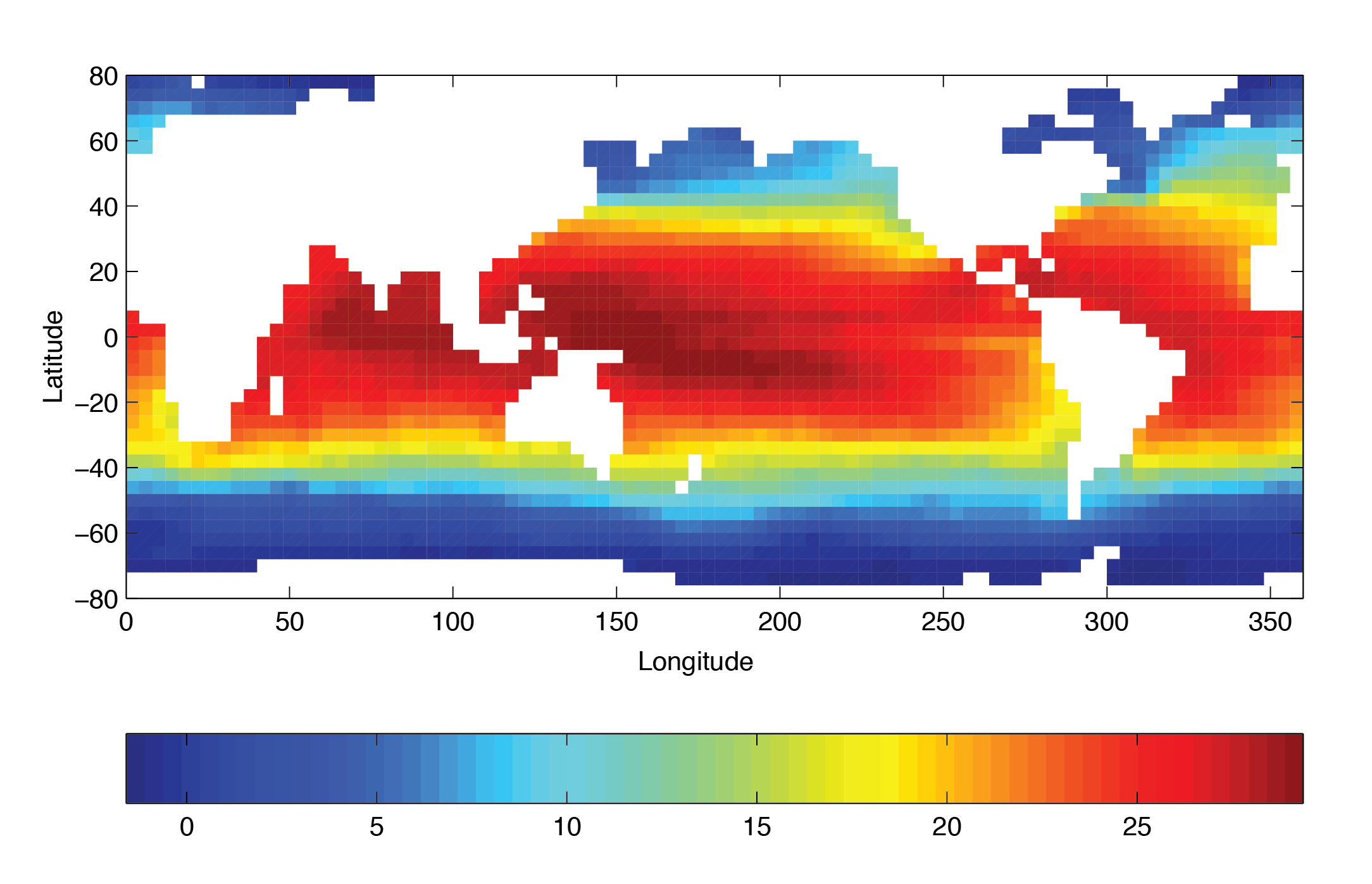
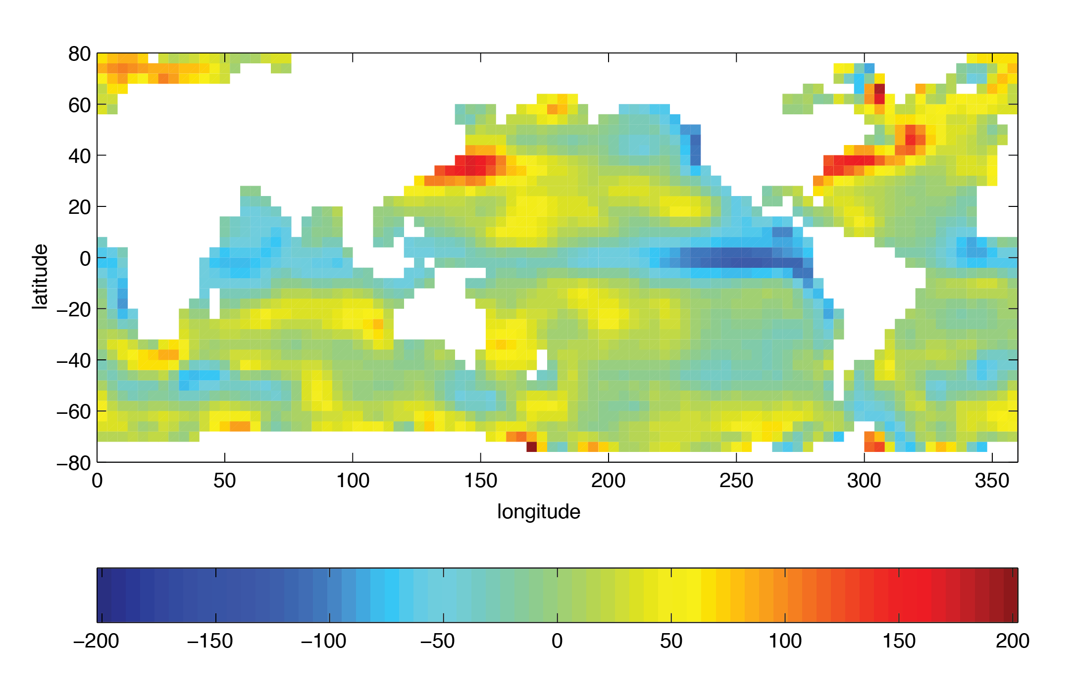
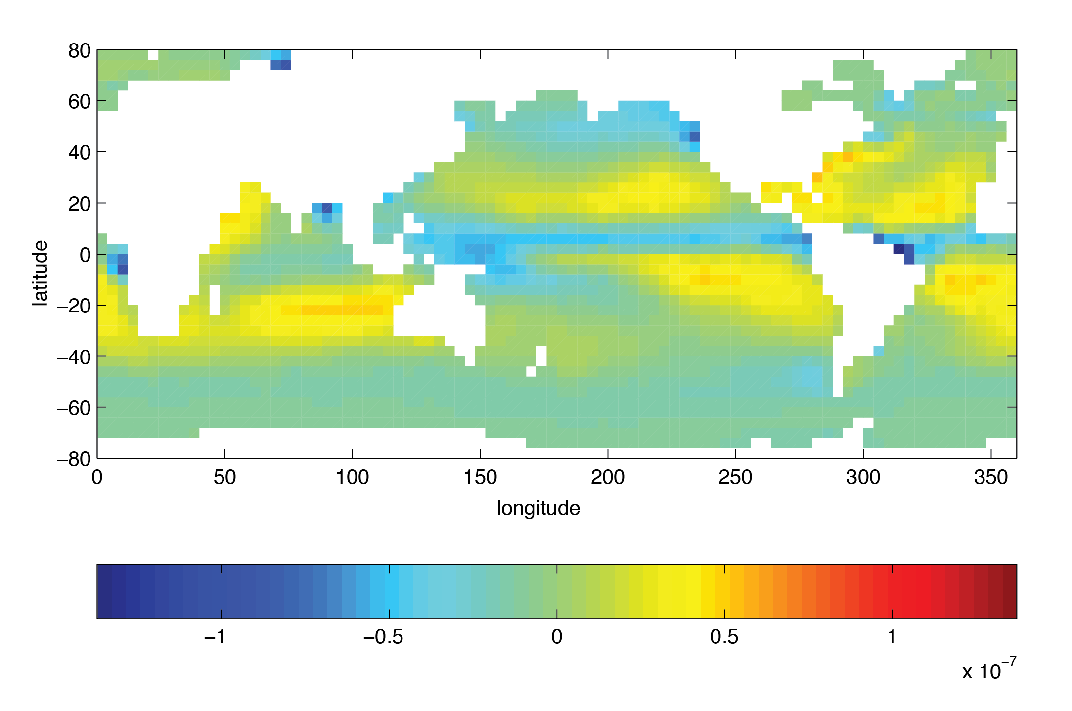
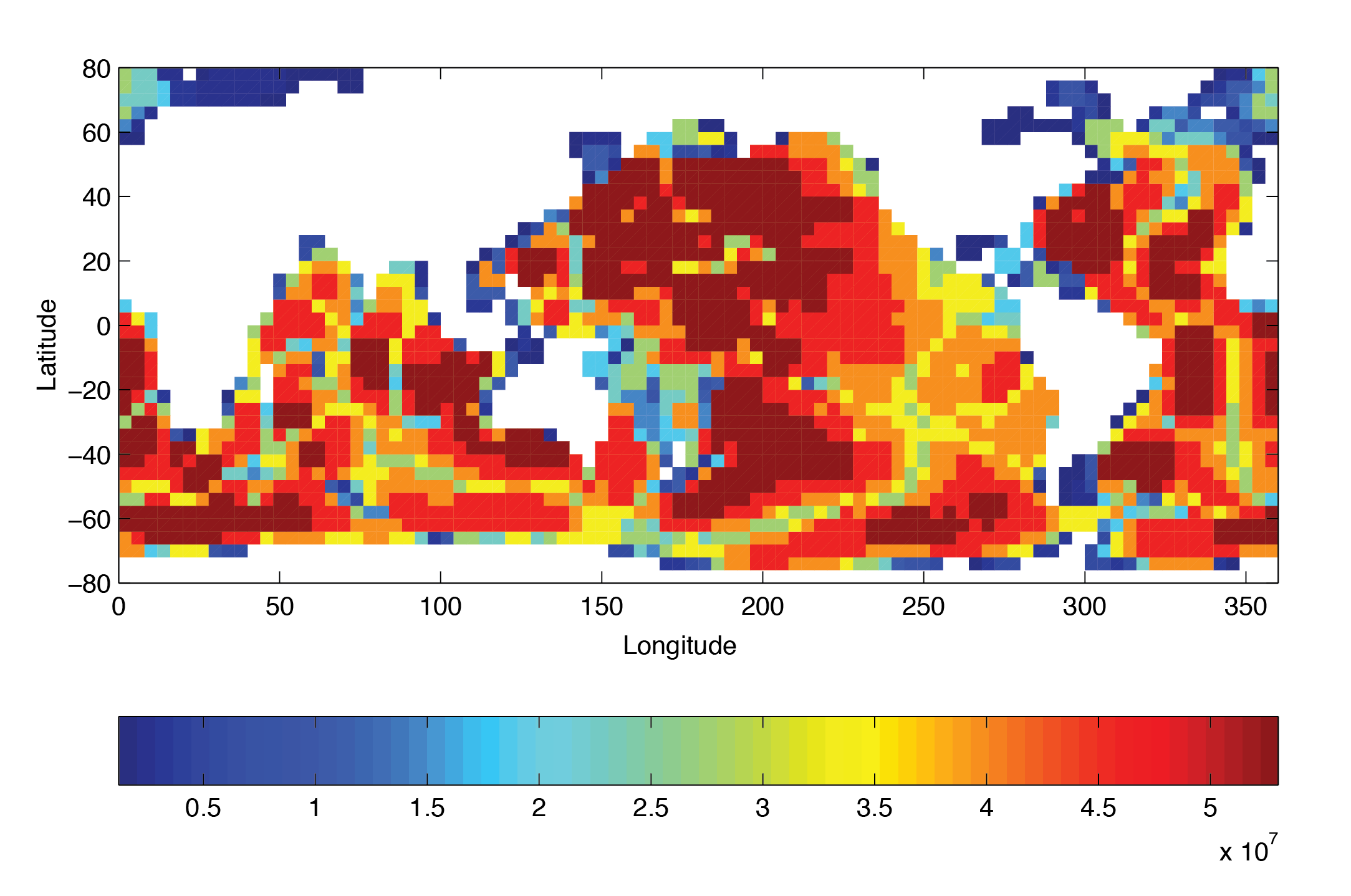
Figure 4.32-Figure 4.37
show the relaxation temperature (\(\theta^{\ast}\)) and salinity
(\(S^{\ast}\)) fields, the wind stress components (\(\tau_x\)
and \(\tau_y\)), the heat flux (\(Q\)) and the net fresh water
flux (\({\cal E} - {\cal P} - {\cal R}\)) used in equations
(4.42) - (4.45).
The figures also indicate the lateral extent and coastline used in the
experiment. Figure 4.38
shows the depth contours of the model domain.
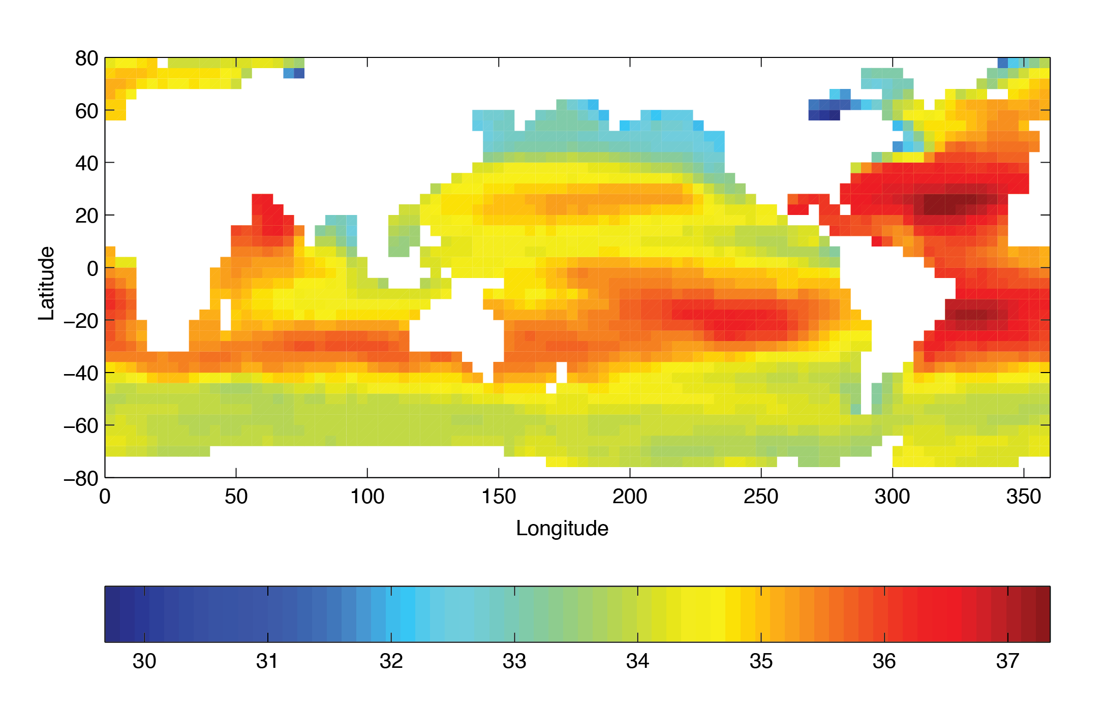
Figure 4.32 Annual mean of relaxation temperature (oC)
Figure 4.33 Annual mean of relaxation salinity (g/kg)
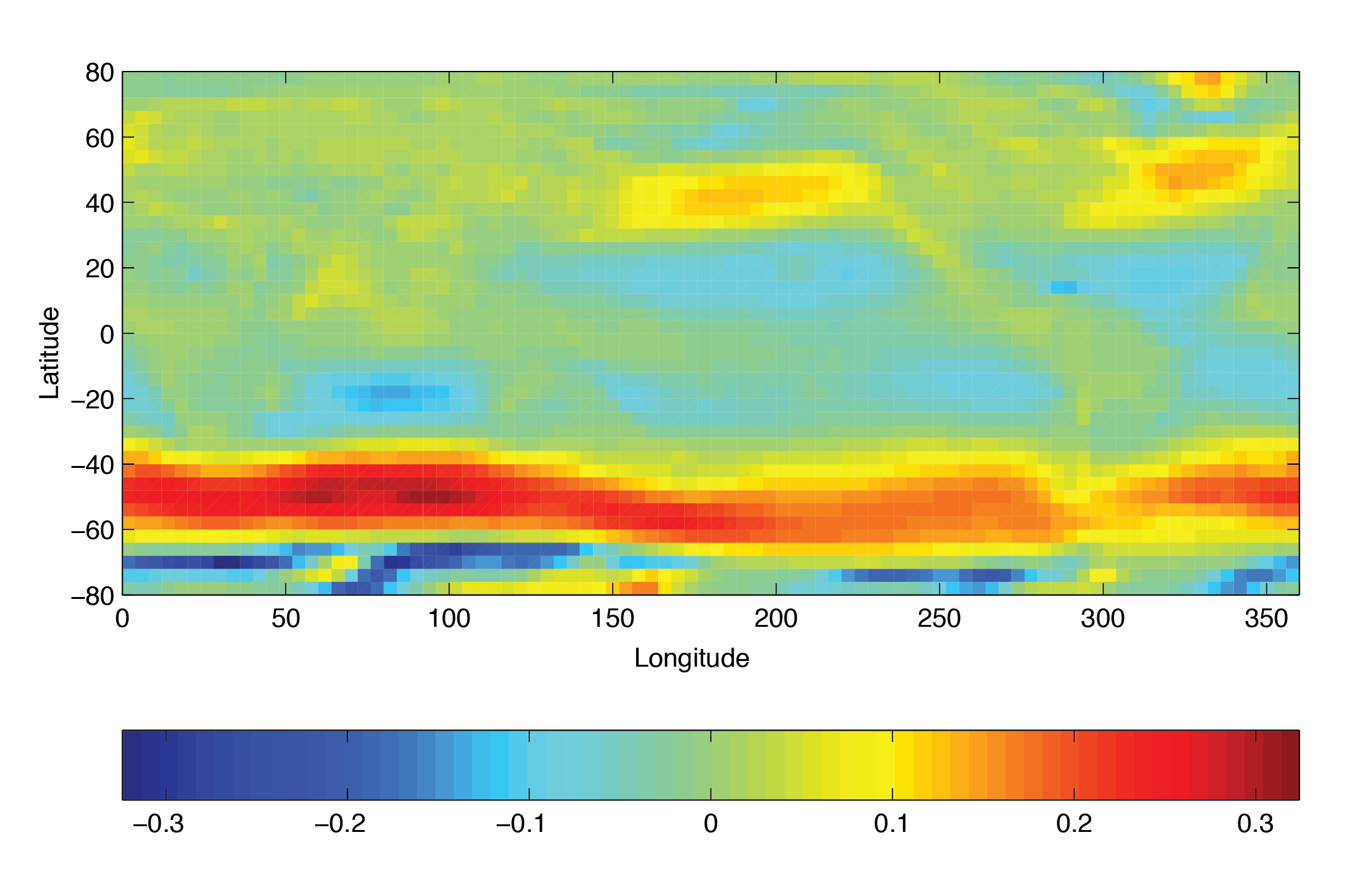
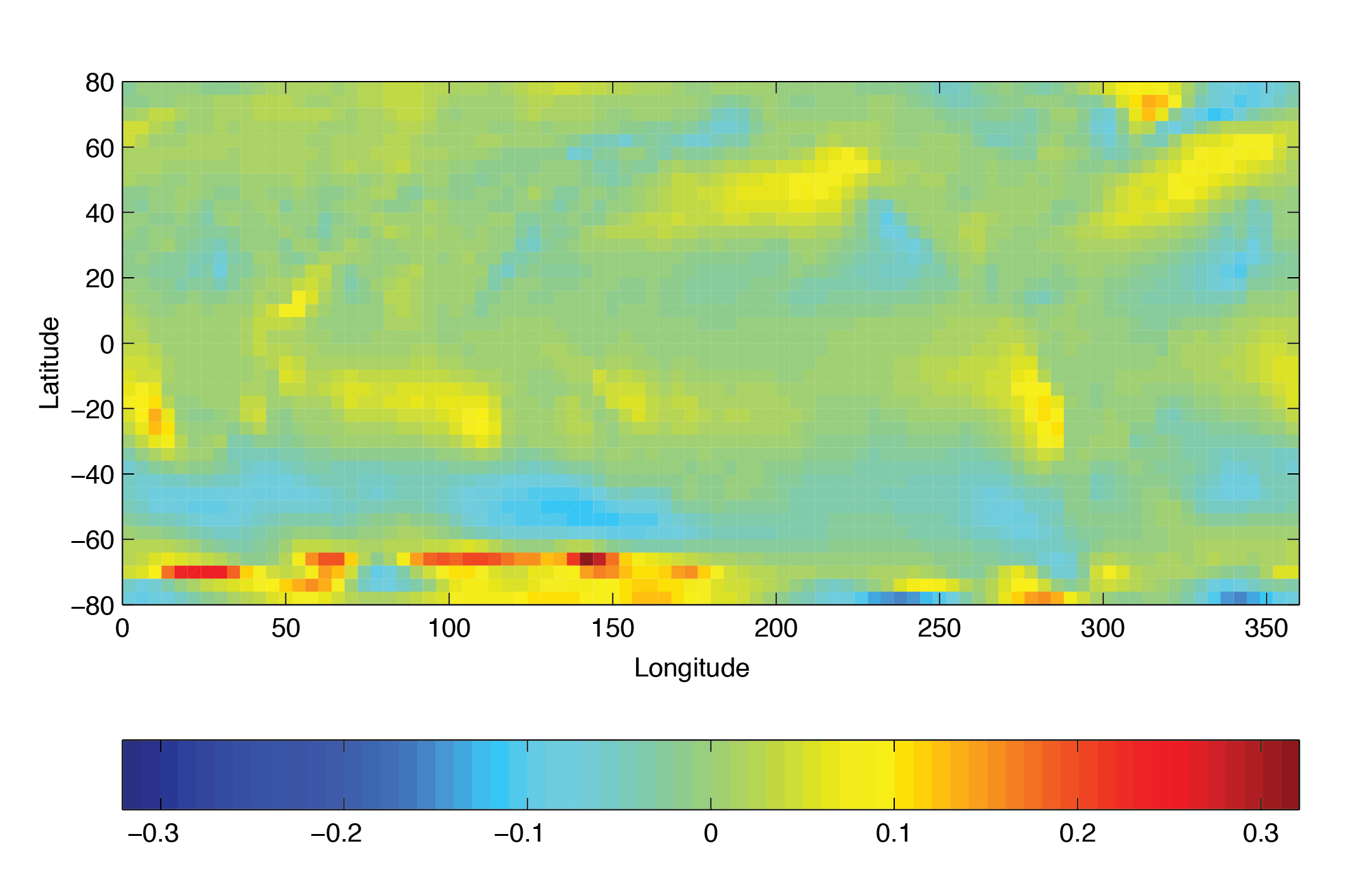
Figure 4.34 Annual mean of zonal wind stress component (N m-2)
Figure 4.35 Annual mean of meridional wind stress component (N m-2)
This file specifies the main parameters
for the experiment. The parameters that are significant for this
configuration are
Line 9–10,
viscAh=3.E5,
no_slip_sides=.TRUE.
these lines set the horizontal Laplacian frictional dissipation
coefficient to \(3 \times 10^{5}\) m2 s-1 and specify
a no-slip boundary condition for this operator, i.e., \(u=0\)
along boundaries in \(y\) and \(v=0\) along boundaries in
\(x\).
These lines set the vertical Laplacian frictional dissipation
coefficient to \(1.721611620915750 \times 10^{5}\) Pa2 s-1,
which corresponds to
\(1.67\times10^{-3}\) m2 s-1 in the commented
line, and specify a free slip boundary condition for this operator, i.e.,
\(\frac{\partial u}{\partial p}=\frac{\partial v}{\partial p}=0\)
at \(p=p_{b}^{0}\), where \(p_{b}^{0}\) is the local bottom
pressure of the domain at rest. Note that the factor
\((g\rho)^2\) needs to be included in this value.
Line 14,
diffKhT=1.E3,
this line sets the horizontal diffusion coefficient for temperature
to 1000 m2 s-1. The boundary condition on this
operator is
\(\frac{\partial}{\partial x}=\frac{\partial}{\partial y}=0\)
on all boundaries.
Line 15–16,
 diffKrT=5.154525811125000e3,
#diffKzT=0.5E-4,
this line sets the vertical diffusion coefficient for temperature to
\(5.154525811125 \times 10^{3}\) Pa2 s-1, which
corresponds to \(5\times10^{-4}\) m2 s-1 in the
commented line. Note that the factor \((g\rho)^2\) needs to be
included in this value. The boundary condition on this operator is
\(\frac{\partial}{\partial p}=0\) at both the upper and lower
boundaries.
Select implicit diffusion as a convection scheme and set coefficient
for implicit vertical diffusion to
\(1.030905162225\times10^{9}\) Pa2 s-1, which corresponds to
10 m2 s-1.
Line 24,
gravity=9.81,
This line sets the gravitational acceleration coefficient to
9.81 m s-1.
Line 25,
rhoConst=1035.,
sets the reference density of sea water to 1035 kg m-3.
Line 29,
eosType='JMD95P',
Selects the full equation of state according to Jackett and McDougall (1995)
[JM95]. Note that the only other sensible choice here could be
the equation of state by McDougall et al. (2003) [MJWF03], MDJFW.
Other model choices for equations of state do not make sense in this
configuration.
Line 28-29,
implicitFreeSurface=.TRUE.,
Selects the barotropic pressure equation to be the implicit free
surface formulation.
Line 32,
exactConserv=.TRUE.,
Select a more accurate conservation of properties at the surface
layer by including the horizontal velocity divergence to update the
free surface.
Line 33–35
nonlinFreeSurf=3,
hFacInf=0.2,
hFacSup=2.0,
Select the nonlinear free surface formulation and set lower and upper
limits for the free surface excursions.
Line 39-40,
readBinaryPrec=64,
writeBinaryPrec=64,
Sets format for reading binary input datasets and writing binary
output datasets containing model fields to use 64-bit representation
for floating-point numbers.
Line 45,
cg2dMaxIters=200,
Sets maximum number of iterations the 2-D conjugate
gradient solver will use, irrespective of convergence criteria
being met.
Line 46,
cg2dTargetResidual=1.E-13,
Sets the tolerance which the 2-D conjugate gradient
solver will use to test for convergence in
(2.15) to
\(1 \times 10^{-9}\). Solver will iterate until tolerance falls
below this value or until the maximum number of solver iterations
is reached.
Line 51,
startTime=0,
Sets the starting time for the model internal time counter. When set
to non-zero, this option implicitly requests a checkpoint file be read
for initial state. By default the checkpoint file is named according
to the integer number of time steps in the startTime value. The
internal time counter works in seconds.
Line 52–54,
endTime=8640000.,
# after 100 years of intergration, one gets a reasonable flow field
#endTime=3110400000.,
Sets the time (in seconds) at which this simulation will terminate.
At the end of a simulation a checkpoint file is automatically written
so that a numerical experiment can consist of multiple stages. The
commented out setting for endTime is for a 100 year simulation.
Sets the timestep \(\delta t_{v}\) used in the momentum
equations to 20 minutes and the timesteps
\(\delta t_{\theta}\) in the tracer equations and
\(\delta t_{\eta}\) in the implicit free surface equation to
48 hours. See Section 2.2.
Line 60,
pChkptFreq =3110400000.,
write a pickup file every 100 years of integration.
write model output and time-averaged model output every 100 years,
and monitor statistics every model time step (this is set for testing purposes; change to a
larger number for long integrations).
Allow periodic external forcing: set one month forcing period during which
a single time slice of data is valid, and the repeat cycle to one
year. Thus, external forcing files will contain twelve periods of forcing data.
These lines specify the names of the files holding the bathymetry
data set, the time-independent geopotential height anomaly at the
bottom, initial conditions of temperature and salinity, wind stress
forcing fields, sea surface temperature climatology, heat flux, and
fresh water flux (evaporation minus precipitation minus runoff) at
the surface. See file descriptions in section
Section 4.6.3.
Other lines in the file input/data
are standard values that are described in the Section 3.8.
This file is a 2-D (\(x,y\)) map of depths. This file is
assumed to contain 64-bit binary numbers giving the depth of the model
at each grid cell, ordered with the \(x\) coordinate varying fastest. The
points are ordered from low coordinate to high coordinate for both axes.
The units and orientation of the depths in this file are the same as
used in the MITgcm code (Pa for this experiment). In this experiment, a
depth of 0 Pa indicates a land point (wall) and a depth of
>0 Pa indicates open ocean.
The file contains twelve identical 2-D maps (\(x,y\)) of
geopotential height anomaly at the bottom at rest. The values have been
obtained by vertically integrating the hydrostatic equation with the
initial density field (using input/lev_t.bin and input/lev_s.bin). This file has to be
consistent with the temperature and salinity field at rest and the choice
of equation of state!
4.6.3.7. Files input/lev_t.bin and input/lev_s.bin
The files input/lev_t.bin and input/lev_s.bin specify the initial conditions for
temperature and salinity for every grid point in a 3-D
array (\(x,y,z\)). The data are obtain by interpolating monthly mean
values using Levitus and Boyer (1994a,b) [LB94a, LB94b] for January onto the model grid.
Keep in mind that the first index corresponds to the bottom layer and
highest index to the surface layer.
4.6.3.8. Files input/trenberth_taux.bin and input/trenberth_tauy.bin
The files input/trenberth_taux.bin and input/trenberth_tauy.bin contain twelve
2-D (\(x,y\)) maps of zonal and meridional wind stress
values, \(\tau_{x}\) and \(\tau_{y}\), respectively, in 3-D arrays (\(x,y,t\)).
These are monthly mean
values from Trenberth et al. (1990) [TOL90], units of N m-2.
The file input/lev_sst.bin contains twelve monthly surface temperature
climatologies from Levitus and Boyer (1994b) [LB94b] in a 3-D
arrays (\(x,y,t\)).
4.6.3.10. Files input/shi_qnet.bin and input/shi_empmr.bin
The files input/shi_qnet.bin and input/shi_empmr.bin contain twelve monthly surface fluxes
of heat (qnet) and freshwater (empmr) from Jiang et al. (1999) [JSMR99] in
3-D arrays (\(x,y,t\)). Both fluxes are normalized so
that the total forcing over one year results in no net flux into the ocean (note, the freshwater
flux is actually constant in time).