This experiment illustrates the optimization capacity of the MITgcm:
here, a high level description.
In this tutorial, a very simple case is used to illustrate the
optimization capacity of the MITgcm. Using an ocean configuration with
realistic geography and bathymetry on a \(4\times4^\circ\) spherical
polar grid, we estimate a time-independent surface heat flux adjustment
\(Q_\mathrm{netm}\) that attempts to bring the model climatology
into consistency with observations (Levitus and Boyer (1994a,b)
[LB94a, LB94b]).
This adjustment \(Q_\mathrm{netm}\) (a 2-D field only function of
longitude and latitude) is the control variable of an optimization
problem. It is inferred by an iterative procedure using an ‘adjoint
technique’ and a least-squares method (see, for example,
Stammer et al. (2002) [SWG+02] and Ferriera et a. (2005) [FMH05].
The ocean model is run forward in time and the quality of the solution
is determined by a cost function, \(J_1\), a measure of the
departure of the model climatology from observations:
where \(\overline{T}_i\) and \(\overline{T}_i^{lev}\) are,
respectively, the model and observed potential temperature at each grid
point \(i\). The differences are weighted by an a priori
uncertainty \(\sigma_i^T\) on observations (as provided by
Levitus and Boyer (1994a)
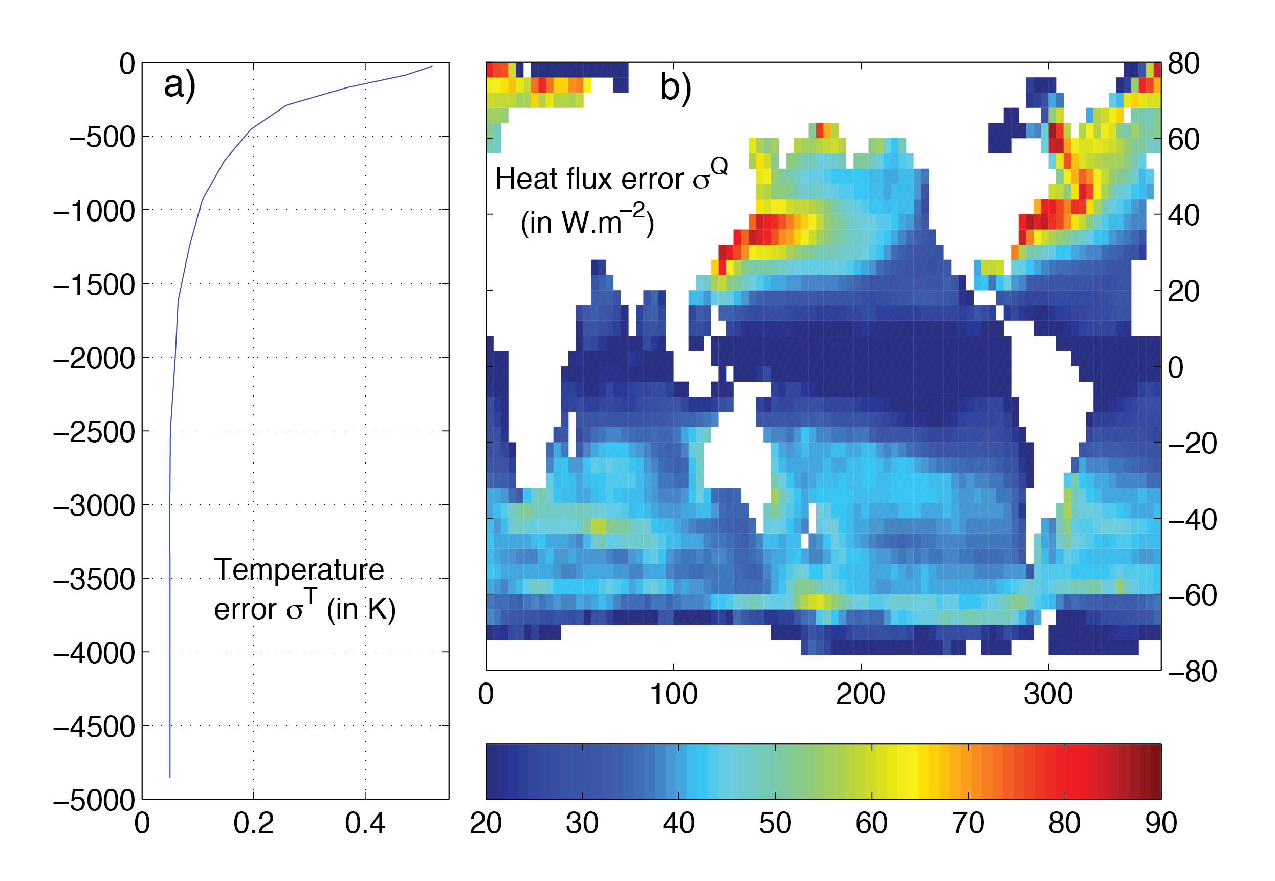
[LB94a]). The error \(\sigma_i^T\) is only a
function of depth and varies from 0.5 K at the surface to 0.05 K at the
bottom of the ocean, mainly reflecting the decreasing temperature
variance with depth (see Figure 4.47a). A value of \(J_1\) of order 1
means that the model is, on average, within observational uncertainties.
Figure 4.47 A priori errors on potential temperature (left, in oC) and surface heat flux
(right, in W m-2) used to compute the cost terms \(J_1\) and \(J_2\), respectively.
The cost function also places constraints on the adjustment to insure it
is “reasonable”, i.e., of order of the uncertainties on the observed
surface heat flux:
where \(\sigma^Q_i\) are the a priori errors on the observed heat
flux as estimated by Stammer et al. (2002) [SWG+02] from 30% of local
root-mean-square variability of the NCEP forcing field (see Figure 4.47b).
The total cost function is defined as
\(J=\lambda_1 J_1+ \lambda_2 J_2\) where \(\lambda_1\) and
\(\lambda_2\) are weights controlling the relative contribution of
the two components. The adjoint model then yields the sensitivities
\(\partial J/\partial Q_\mathrm{netm}\) of \(J\) relative to the
2-D fields \(Q_\mathrm{netm}\). Using a line-searching algorithm
(Gilbert and Lemaréchal 1989 [GLemarechal89]), \(Q_\mathrm{netm}\) is adjusted
then in the sense to reduce \(J\) — the procedure is repeated until
convergence.
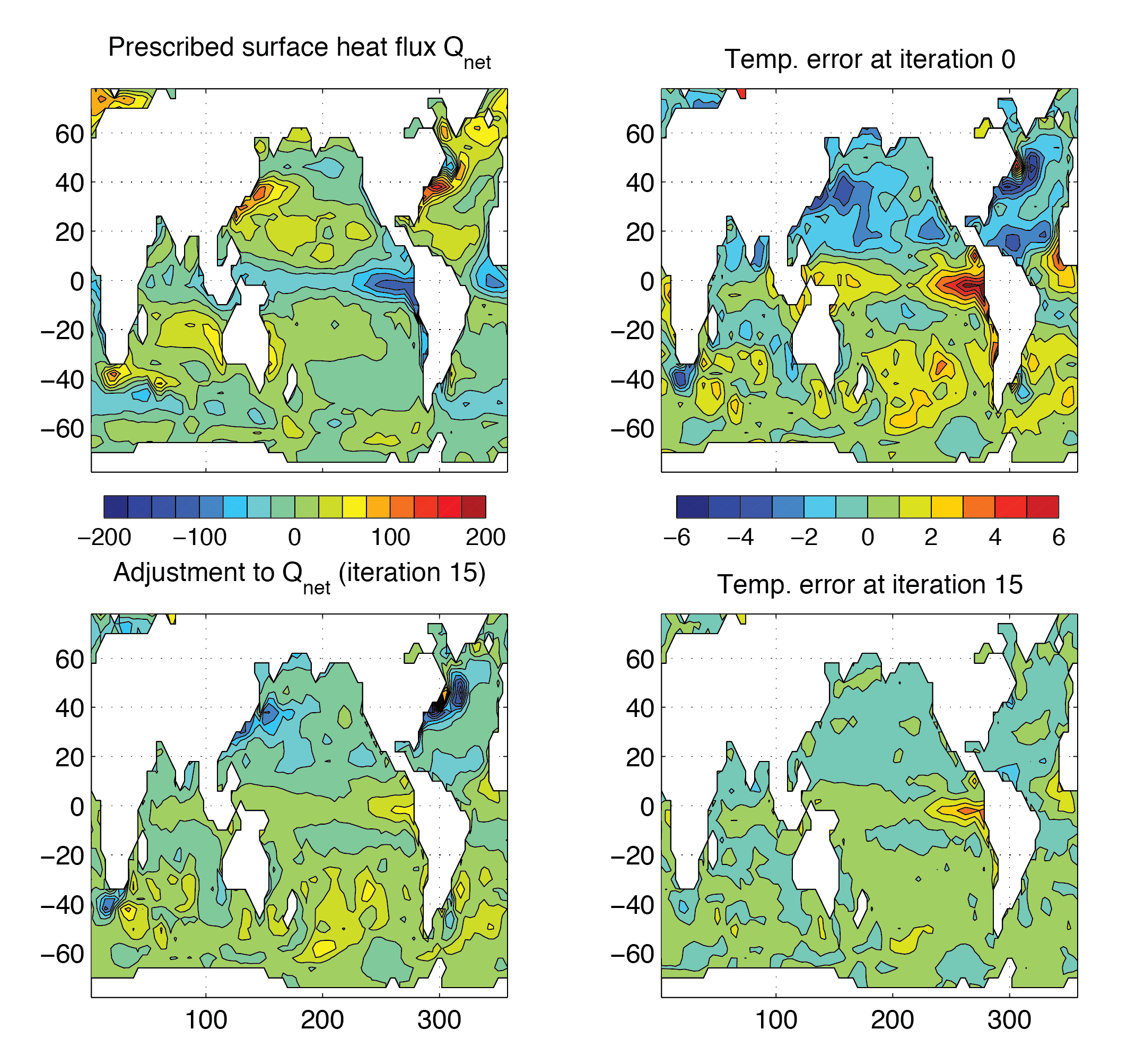
Figure 4.48 shows the results of such an optimization. The model is
started from rest and from January-mean temperature and salinity initial
conditions taken from the Levitus dataset. The experiment is run a year
and the averaged temperature over the whole run (i.e., annual mean) is
used in the cost function (4.58) to evaluate the model 1.
Only the top 2 levels are used. The first guess \(Q_\mathrm{netm}\)
is chosen to be zero. The weights \(\lambda_1\) and
\(\lambda_2\) are set to 1 and 2, respectively. The total cost
function converges after 15 iterations, decreasing from 6.1 to 2.7 (the
temperature contribution decreases from 6.1 to 1.8 while the heat flux
one increases from 0 to 0.42). The right panels of Figure 4.48
illustrate the evolution of the temperature error at the surface from
iteration 0 to iteration 15. Unsurprisingly, the largest errors at
iteration 0 (up to 6 oC, top left panels) are found in
the Western boundary currents. After optimization, the departure of the
model temperature from observations is reduced to 1 oC
or less almost everywhere except in the Pacific equatorial cold tongue.
Comparison of the initial temperature error (top, right) and heat flux
adjustment (bottom, left) shows that the system basically increased the
heat flux out of the ocean where temperatures were too warm and
vice-versa. Obviously, heat flux uncertainties are not solely
responsible for temperature errors, and the heat flux adjustment partly
compensates the poor representation of narrow currents (Western boundary
currents, equatorial currents) at \(4\times4^\circ\) resolution.
This is allowed by the large a priori error on the heat flux Figure 4.47.
The Pacific cold tongue is a counter example: there, heat
fluxes uncertainties are fairly small (about 20 W m-2), and a
large temperature errors remains after optimization.
Figure 4.48 Initial annual mean surface heat flux (top right in W m-2) and adjustment obtained at iteration 15 (bottom right).
Averaged difference between model and observed potential temperatures at the surface (in \(^\circ\)C)
before optimization (iteration 0, top right) and after optimization (iteration 15, bottom right).
Contour intervals for heat flux and temperature are 25 W m-2 and 1 oC, respectively. A positive flux is out of the ocean.
4.11.2. Implementation of the control variable and the cost function
One of the goals of this tutorial is to illustrate how to implement a new
control variable. Most of this is fairly generic and is done in pkg/ctrl
and pkg/cost. The modifications can be
tracked by the CPP option ALLOW_HFLUXM_CONTROL or the comment
cHFLUXM_CONTROL. The more specific modifications required for the
experiment are found in
verification/tutorial_global_oce_optim/code_ad. Here follows a brief
description of the implementation.
pkg/ctrl/ctrl_init.F where \(Q_\mathrm{netm}\) is defined as the control
variable number 24,
pkg/ctrl/ctrl_pack.F which writes, at the end of each iteration, the
sensitivity of the cost function
\(\partial J/\partial Q_\mathrm{netm}\) in to a file to be used
by the line-search algorithm,
pkg/ctrl/ctrl_unpack.F which reads, at the start of each iteration, the
updated adjustment as provided by the line-search algorithm,
pkg/ctrl/ctrl_map_forcing.F in which the updated adjustment is added to the
first guess \(Q_\mathrm{netm}\).
input_ad/data.ctrl is used, in particular, to specify the name of the
sensitivity and adjustment files associated to a control variable,
input_ad/data.cost: parameters of the cost functions, in particular
lastinterval specifies the length of time-averaging for the model
temperature to be used in the cost function (4.58),
% ../../../tools/genmake2 -mods=../code_ad -adof=../code_ad/ad_optfile.local
% make depend
% make adall
to generate the MITgcm executable mitgcmuv_ad.
4.11.4.2. Compilation of the line-search algorithm: optim.x
This is done from the directories lsopt/ and optim/ (found in the top MITgcm directory). In
lsopt/, unzip the blash1 library adapted to your platform (see lsopt/README), and change
the Makefile accordingly. Compile with:
In optim/, the path of the directory where mitgcm_ad was compiled
must be specified in the Makefile in the variable INCLUDEDIRS. The file
name of the control variable (here, xx_hfluxm_file) must be added to
the namelist read by optim/optim_numbmod.F. Then use
Make a new subdirectory input_ad/OPTIM.
Copy the mitgcmuv_ad executable to input_ad
and optim.x to this subdirectory.
cd into input_ad/. The first iteration
is somewhat particular and is best done “by hand” while the following
iterations can be run automatically (see below). Check that the
iteration number is set to 0 in input_ad/data.optim and run MITgcm:
% ./mitgcmuv_ad
The output files adxx_hfluxm.0000000000.* and xx_hfluxm.0000000000.*
contain the sensitivity of the cost function to \(Q_\mathrm{netm}\)
and the adjustment to \(Q_\mathrm{netm}\) (zero at the first
iteration), respectively. Two other files called
costhflux_tut_MITgcm.opt0000 and ctrlhflux_tut_MITgcm.opt0000 are
also generated. They essentially contain the same information as the
adxx_.hfluxm* and xx_hfluxm* files, but in a compressed format.
These two files are the only ones involved in the communication between
the adjoint model mitgcmuv_ad and the line-search algorithm
optim.x. Only at the first iteration, are they both generated by
mitgcmuv_ad. Subsequently, costhflux_tut_MITgcm.opt\(n\) is
an output of the adjoint model at iteration \(n\) and an input of
the line-search. The latter returns an updated adjustment in
ctrlhflux_tut_MITgcm.opt\(n+1\) to be used as an input of the
adjoint model at iteration \(n+1\).
At the first iteration, move costhflux_tut_MITgcm.opt0000 and
ctrlhflux_tut_MITgcm.opt0000 to input_ad/OPTIM,
move into this directory and link input_ad/data.optim
and input_ad/data.ctrl locally:
The target cost function fmin needs to be specified
in input_ad/data.optim: as a rule of
thumb, it should be about 0.95-0.90 times the value of the cost function
at the first iteration. This value is only used at the first iteration
and does not need to be updated afterward. However, it implicitly
specifies the “pace” at which the cost function is going down (if you
are lucky and it does indeed diminish!).
Once this is done, run the line-search algorithm:
% ./optim.x
which computes the updated adjustment for iteration 1,
ctrlhflux_tut_MITgcm.opt0001.
The following iterations can be executed automatically using the shell
script input_ad/cycsh. This script will take care of
changing the iteration numbers in input_ad/data.optim, launch the adjoint
model, clean and store the outputs, move the costhflux* and ctrlhflux*
files, and run the line-search algorithm. Edit input_ad/cycsh to specify the
prefix of the directories used to store the outputs and the maximum
number of iteration.
Because of the daily automatic testing, the experiment as found in
the repository is set-up with a very small number of time-steps. To
reproduce the results shown here, one needs to set nTimeSteps = 360
and lastinterval =31104000 (both corresponding to a year, see Section 4.11.3.2 for further details).