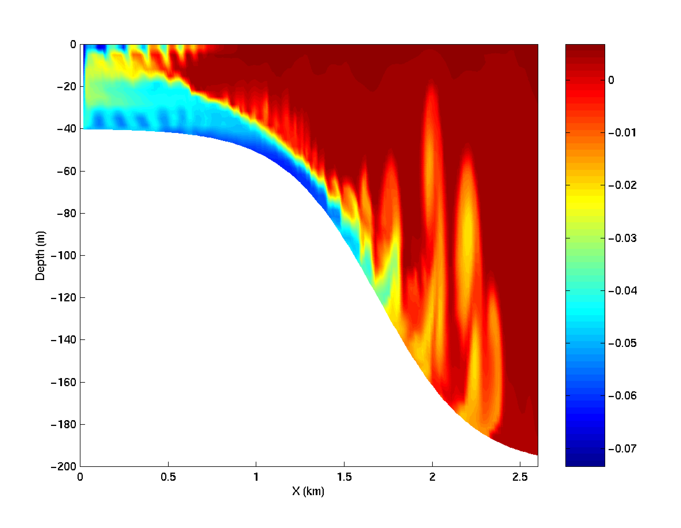
Figure 4.42 Temperature after 23 hours of cooling. The cold dense water is mixed with ambient water as it accelerates down the slope and hence is warmer than the unmixed plume.
An important test of any ocean model is the ability to represent the
flow of dense fluid down a slope. One example of such a flow is a
non-rotating gravity plume on a continental slope, forced by a limited
area of surface cooling above a continental shelf. Because the flow is
non-rotating, a two dimensional model can be used in the across slope
direction. The experiment is non-hydrostatic and uses open-boundaries to
radiate transients at the deep water end. (Dense flow down a slope can
also be forced by a dense inflow prescribed on the continental shelf;
this configuration is being implemented by the DOME (Dynamics of
Overflow Mixing and Entrainment) collaboration to compare solutions in
different models).
The fluid is initially unstratified. The surface buoyancy loss
\(B_0\) (dimensions of L\(^2\)T\(^{-3}\)) over a
cross-shelf distance \(R\) causes vertical convective mixing and
modifies the density of the fluid by an amount
\[\Delta \rho = \frac{B_0 \rho_0 t}{g H}\]
where \(H\) is the depth of the shelf, \(g\) is the
acceleration due to gravity, \(t\) is time since onset of cooling
and \(\rho_0\) is the reference density. Dense fluid slumps under
gravity, with a flow speed close to the gravity wave speed:
The Froude number of the flow on the shelf is close to unity (but in
practice slightly less than unity, giving subcritical flow). When the
flow reaches the slope, it accelerates, so that it may become
supercritical (provided the slope angle \(\alpha\) is steep
enough). In this case, a hydraulic control is established at the shelf
break. On the slope, where the Froude number is greater than one, and
gradient Richardson number (defined as \(Ri \sim g' h^*/U^2\) where
\(h^*\) is the thickness of the interface between dense and ambient
fluid) is reduced below 1/4, Kelvin-Helmholtz instability is possible,
and leads to entrainment of ambient fluid into the plume, modifying the
density, and hence the acceleration down the slope. Kelvin-Helmholtz
instability is suppressed at low Reynolds and Peclet numbers given by
\[Re \sim \frac{U h}{ \nu} \sim \frac{(B_0 R)^{1/3} h}{\nu} \mbox{ ; } Pe = Re Pr\]
where \(h\) is the depth of the dense fluid on the slope. Hence
this experiment is carried out in the high Re, Pe regime. A further
constraint is that the convective heat flux must be much greater than
the diffusive heat flux (Nusselt number \(\gg 1\)). Then
\[Nu = \frac{U h^* }{\kappa} \gg 1\]
Finally, since we have assumed that the convective mixing on the shelf
occurs in a much shorter time than the horizontal equilibration, this
implies \(H/R \ll 1\).
Hence to summarize the important non-dimensional parameters, and the
limits we are considering:
\[\frac{H}{R} \ll 1 \mbox{ ; } Re \gg 1 \mbox{ ; } Pe \gg 1 \mbox{ ; } Nu \gg 1
\mbox{ ; } \mbox{ ; } Ri < 1/4 .\]
In addition we are assuming that the slope is steep enough to provide
sufficient acceleration to the gravity plume, but nonetheless much less
that 1:1, since many Kelvin-Helmholtz billows appear on the
slope, implying horizontal length scale of the slope \(\gg\) the depth
of the dense fluid.
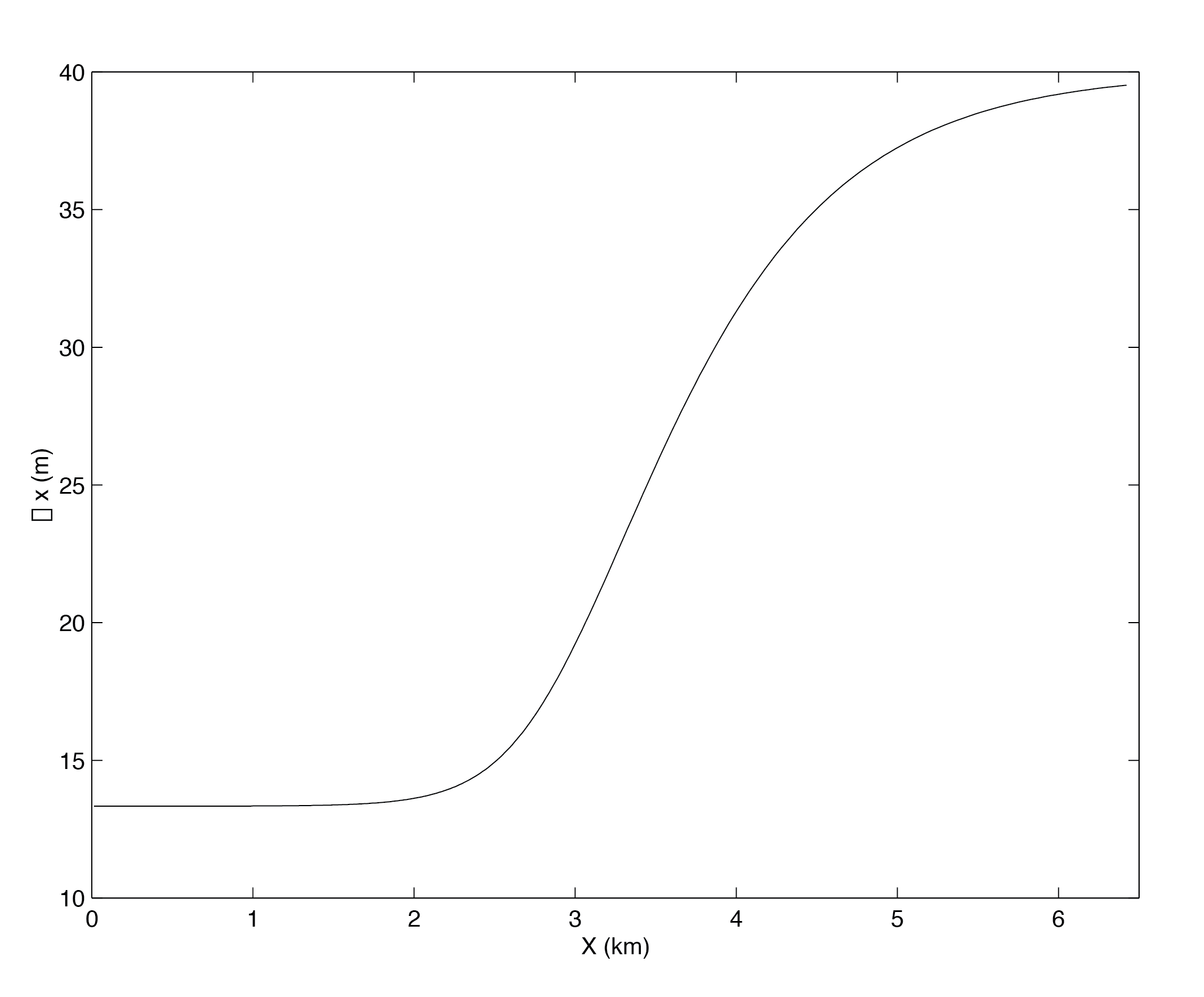
Figure 4.43 Horizontal grid spacing, \(\Delta x\), in the across-slope direction for the gravity plume experiment.
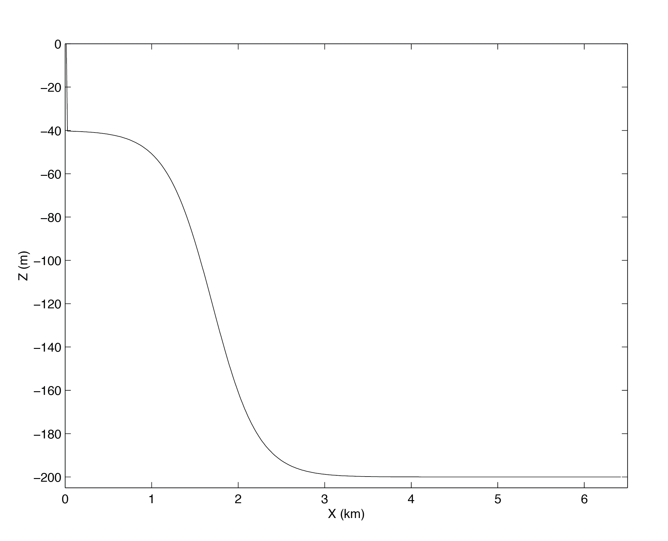
Figure 4.44 Topography, \(h(x)\), used for the gravity plume experiment.
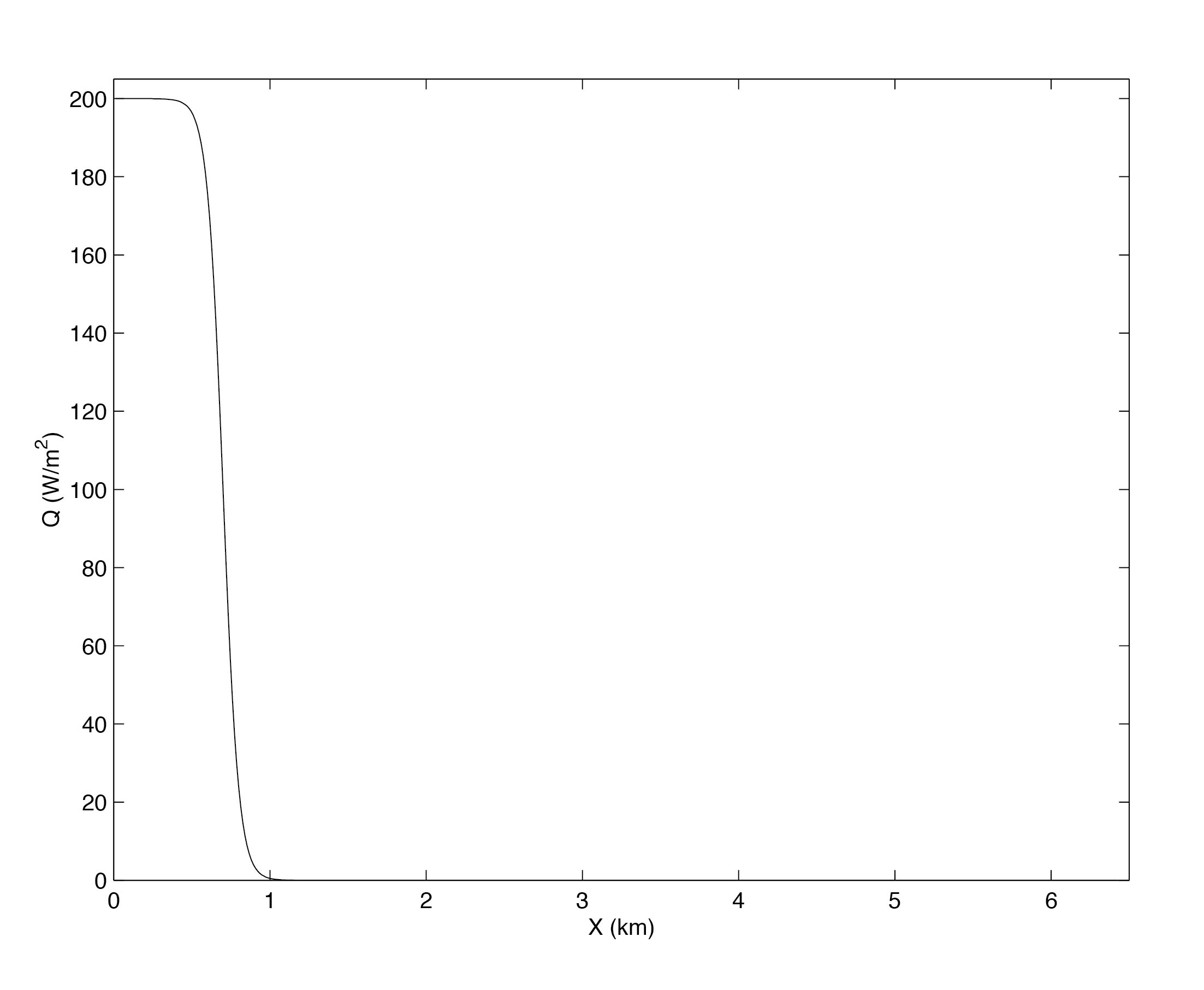
Figure 4.45 Upward surface heat flux, \(Q(x)\), used as forcing in the gravity plume experiment.
The domain is \(200\) m deep and \(6.4\) km across. Uniform
resolution of \(60\times3^1/_3\) m is used in the vertical and
variable resolution of the form shown in Figure 4.43
with 320 points is used in the horizontal. The formula for
\(\Delta x\) is:
Here, \(\Delta x_1\) is the resolution on the shelf,
\(\Delta x_2\) is the resolution in deep water and \(Nx\) is the
number of points in the horizontal.
The topography, shown in Figure 4.44, is given by:
Here, \(s\) is the maximum slope, \(H_o\) is the maximum depth,
\(h_s\) is the shelf depth, \(x_s\) is the lateral position of
the shelf-break and \(L_s\) is the length-scale of the slope.
The forcing is through heat loss over the shelf, shown in
Figure 4.45 and takes the form of a fixed flux with
profile:
Here, \(Q_o\) is the maximum heat flux, \(x_q\) is the
position of the cut-off, and \(L_q\) is the width of the cut-off.
The initial temperature field is unstratified but with random
perturbations, to induce convection early on in the run. The random
perturbation are calculated in computational space and because of the
variable resolution introduce some spatial correlations, but this does
not matter for this experiment. The perturbations have range
\(0-0.01\)\(^{\circ}\mathrm{K}\).
The computational domain (number of gridpoints) is specified in
code/SIZE.h
and is configured as a single tile of dimensions
\(320\times1\times60\).
To compile the model code for this experiment, the non-hydrostatic
algorithm needs to be enabled, and the open-boundaries package (pkg/obcs) is required:
Open boundaries are enabled by adding line obcs to package
configuration file code/packages.conf
and activated via
useOBCS=.TRUE, in namelist PACKAGES
of input/data.pkg.
Table 4.1 Model parameters used in the gravity plume experiment.
Parameter
Value
Description
\(g\)
9.81 m s-2
acceleration due to gravity
\(\rho_o\)
999.8 kg m-3
reference density
\(\alpha\)
2 \(\times\) 10-4 K-1
expansion coefficient
\(A_h\)
1 \(\times\) 10-2 m2 s-1
horizontal viscosity
\(A_v\)
1 \(\times\) 10-3 m2 s-1
vertical viscosity
\(\kappa_h\)
0 m2 s-1
(explicit) horizontal diffusion
\(\kappa_v\)
0 m2 s-1
(explicit) vertical diffusion
\(\Delta t\)
20 s
time step
\(\Delta z\)
3.33333 m
vertical grid spacing
\(\Delta x\)
13.3333 - 39.5 m
horizontal grid spacing
The model parameters (Table 4.1) are specified in
input/data
and if not assume the default values as defined in Section 3.8.
A linear equation of state is used,
eosType=’LINEAR’, but only temperature is active, sBeta=0.E-11.
For the given heat flux, \(Q_o\), the buoyancy forcing is
\(B_o = \frac{g \alpha Q}{\rho_o c_p} \sim
10^{-7}\) m2 s-3. Using \(R=10^3\) m, the
shelf width, this gives a velocity scale of
\(U\sim 5 \times 10^{-2}\) m s-1 for the initial front but
will accelerate by an order of magnitude over the slope. The temperature
anomaly will be of order \(\Delta \theta \sim 3
\times 10^{-2}\) K. The viscosity is constant and gives a Reynolds number
of \(100\), using \(h=20\) m for the initial front and will be
an order magnitude bigger over the slope. There is no explicit diffusion
but a non-linear advection scheme is used for temperature which adds
enough diffusion so as to keep the model stable. The time-step is set to
\(20\) s and gives Courant number order one when the flow reaches
the bottom of the slope.