This example experiment demonstrates using the MITgcm to simulate the
planetary ocean circulation. The simulation is configured with
realistic geography and bathymetry on a
\(4^{\circ} \times 4^{\circ}\) spherical polar grid. Fifteen levels are used in the
vertical, ranging in thickness from 50 m at the surface to 690 m at depth, giving a
maximum model depth of 5200 m. Different time-steps are
used to accelerate the convergence to equilibrium (see Bryan 1984 [Bry84])
so that, at this resolution, the
configuration can be integrated forward for thousands of years on a
single processor desktop computer.
The model is forced with climatological wind stress data from Trenberth (1990)
[TOL90] and NCEP surface flux data from Kalnay et al. (1996)
[KKK+96]. Climatological data (Levitus and Boyer 1994a,b [LB94a, LB94b])
is used to initialize the model
hydrography. Levitus and Boyer seasonal climatology
data is also used throughout the calculation to provide additional
air-sea fluxes. These fluxes are combined with the NCEP climatological
estimates of surface heat flux, resulting in a mixed boundary condition
of the style described in Haney (1971) [Han71]. Altogether, this
yields the following forcing applied in the model surface layer.
where \({\cal F}_{u}\), \({\cal F}_{v}\),
\({\cal F}_{\theta}\), \({\cal F}_{s}\) are the forcing terms in
the zonal and meridional momentum and in the potential temperature and
salinity equations respectively. The term \(\Delta z_{s}\)
represents the top ocean layer thickness in meters. It is used in
conjunction with a reference density, \(\rho_{0}\) (here set to
999.8 kg m-3), a reference salinity, \(S_{0}\)
(here set to 35 ppt), and a specific heat capacity, \(C_{p}\) (here
set to 4000 J kg-1 K-1), to
convert input dataset values into time tendencies of potential
temperature (with units of oC s-1),
salinity (with units ppt s-1) and velocity (with units
m s-2). The externally supplied forcing fields
used in this experiment are \(\tau_{x}\), \(\tau_{y}\),
\(\theta^{\ast}\), \(S^{\ast}\), \(\cal{Q}\) and
\(\mathcal{E}-\mathcal{P}-\mathcal{R}\). The wind stress fields (\(\tau_x\),
\(\tau_y\)) have units of N m-2. The
temperature forcing fields (\(\theta^{\ast}\) and \(Q\)) have
units of oC and W m-2
respectively. The salinity forcing fields (\(S^{\ast}\) and
\(\cal{E}-\cal{P}-\cal{R}\)) have units of ppt and
m s-1 respectively. The source files and
procedures for ingesting this data into the simulation are described in
the experiment configuration discussion in section
Section 4.5.3.
The model is configured in hydrostatic form. The domain is discretized
with a uniform grid spacing in latitude and longitude on the sphere
\(\Delta \phi=\Delta \lambda=4^{\circ}\), so that there are 90
grid cells in the zonal and 40 in the meridional direction. The
internal model coordinate variables \(x\) and \(y\) are
initialized according to
\[ \begin{align}\begin{aligned}x &= r\cos(\phi), &\Delta x & = r\cos(\Delta \phi)\\y &= r\lambda, &\Delta y &= r\Delta \lambda\end{aligned}\end{align} \]
Arctic polar regions are not included in this experiment. Meridionally
the model extends from 80oS to
80oN. Vertically the model is configured with
fifteen layers with the following thicknesses:
\(\Delta z_{1}\) = 50 m
\(\Delta z_{2}\) = 70 m
\(\Delta z_{3}\) = 100 m
\(\Delta z_{4}\) = 140 m
\(\Delta z_{5}\) = 190 m
\(\Delta z_{6}\) = 240 m
\(\Delta z_{7}\) = 290 m
\(\Delta z_{8}\) = 340 m
\(\Delta z_{9}\) = 390 m
\(\Delta z_{10}\) = 440 m
\(\Delta z_{11}\) = 490 m
\(\Delta z_{12}\) = 540 m
\(\Delta z_{13}\) = 590 m
\(\Delta z_{14}\) = 640 m
\(\Delta z_{15}\) = 690 m
(here the numeric subscript indicates the model level index number,
\({\tt k}\)) to give a total depth, \(H\), of
-5200 m. The implicit free surface form of the pressure
equation described in Marshall et al. (1997) [MHPA97] is employed. A
Laplacian operator, \(\nabla^2\), provides viscous dissipation.
Thermal and haline diffusion is also represented by a Laplacian
operator.
Wind-stress forcing is added to the momentum equations in
(4.34) for both the zonal
flow \(u\) and the meridional flow \(v\), according to
equations (4.30) and (4.31). Thermodynamic
forcing inputs are added to the equations in
(4.35) for potential
temperature, \(\theta\), and salinity, \(S\), according to equations
(4.32) and (4.33). This produces a set
of equations solved in this configuration as follows:
where \(u=\frac{Dx}{Dt}=r \cos(\phi)\frac{D \lambda}{Dt}\) and
\(v=\frac{Dy}{Dt}=r \frac{D \phi}{Dt}\) are the zonal and
meridional components of the flow vector, \(\vec{\bf u}\), on the
sphere. As described in Section 2, the time evolution of
potential temperature \(\theta\) equation is solved
prognostically. The total pressure \(p\) is diagnosed by summing
pressure due to surface elevation \(\eta\) and the hydrostatic
pressure.
The Laplacian dissipation coefficient, \(A_{h}\), is set to
\(5 \times 10^5\) m s-1. This value is chosen to yield a Munk
layer width (see Adcroft 1995 [Adc95]),
of ~600 km. This is greater than
the model resolution in low-latitudes,
\(\Delta x \approx\) 400 km, ensuring that the frictional
boundary layer is adequately resolved.
The model is stepped forward with a time step
\(\Delta
t_{\theta}\) = 24 hours for thermodynamic variables and
\(\Delta t_{v}\) = 30 minutes for momentum terms. With this time step, the
stability parameter to the horizontal Laplacian friction
(Adcroft 1995 [Adc95])
evaluates to 0.6 at a latitude of
\(\phi\) = 80o, which is above the 0.3 upper limit for
stability, but the zonal grid spacing \(\Delta x\) is smallest at
\(\phi\) = 80o where \(\Delta
x=r\cos(\phi)\Delta \phi\approx\) 77 km and the stability criterion
is already met one grid cell equatorwards (at \(\phi\) = 76o).
The vertical dissipation coefficient,
\(A_{z}\), is set to \(1\times10^{-3}\) m2 s-1.
The associated stability limit
contain the code customizations and parameter settings for these
experiments. Below we describe the customizations to these files
associated with this experiment.
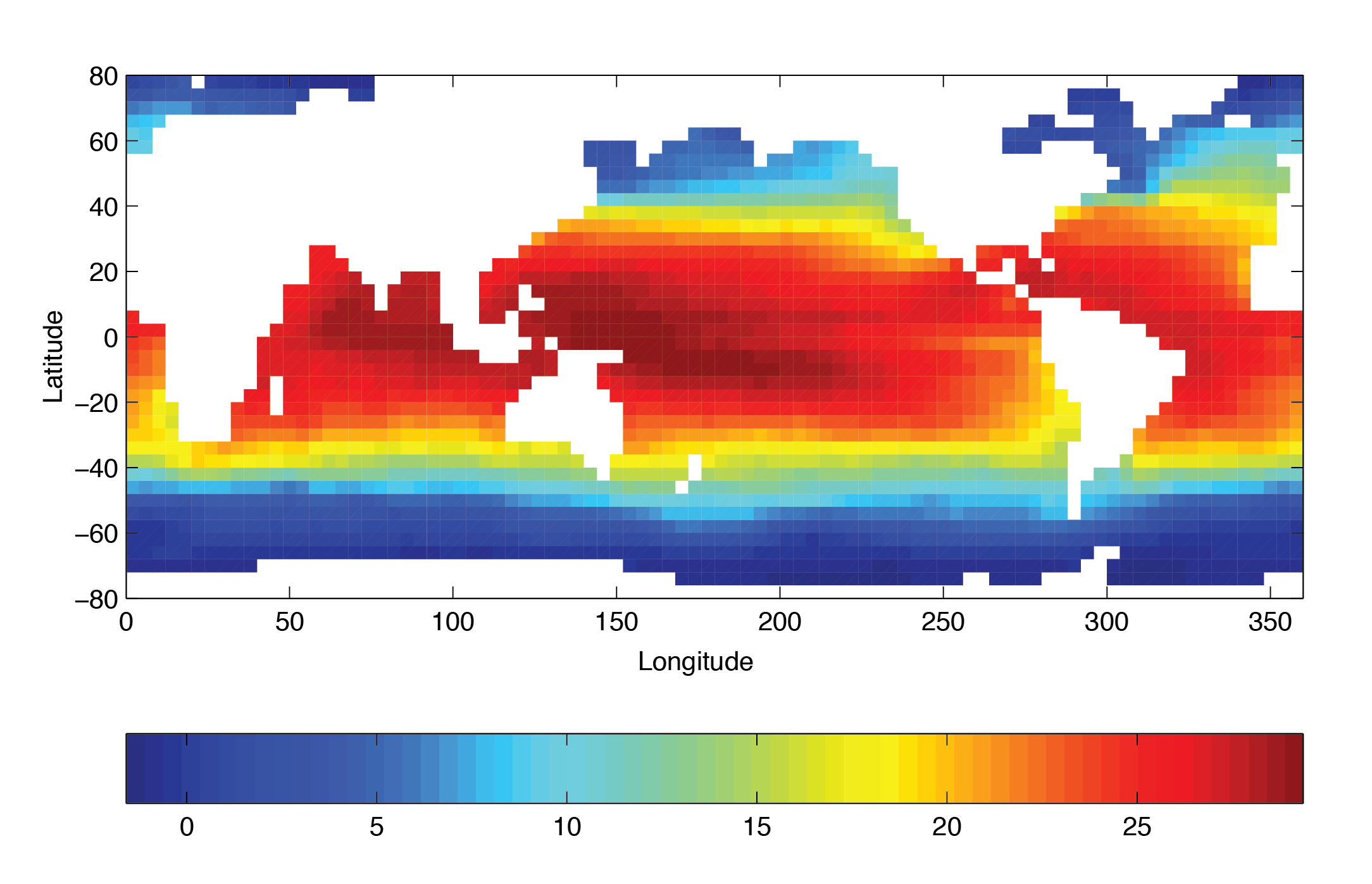
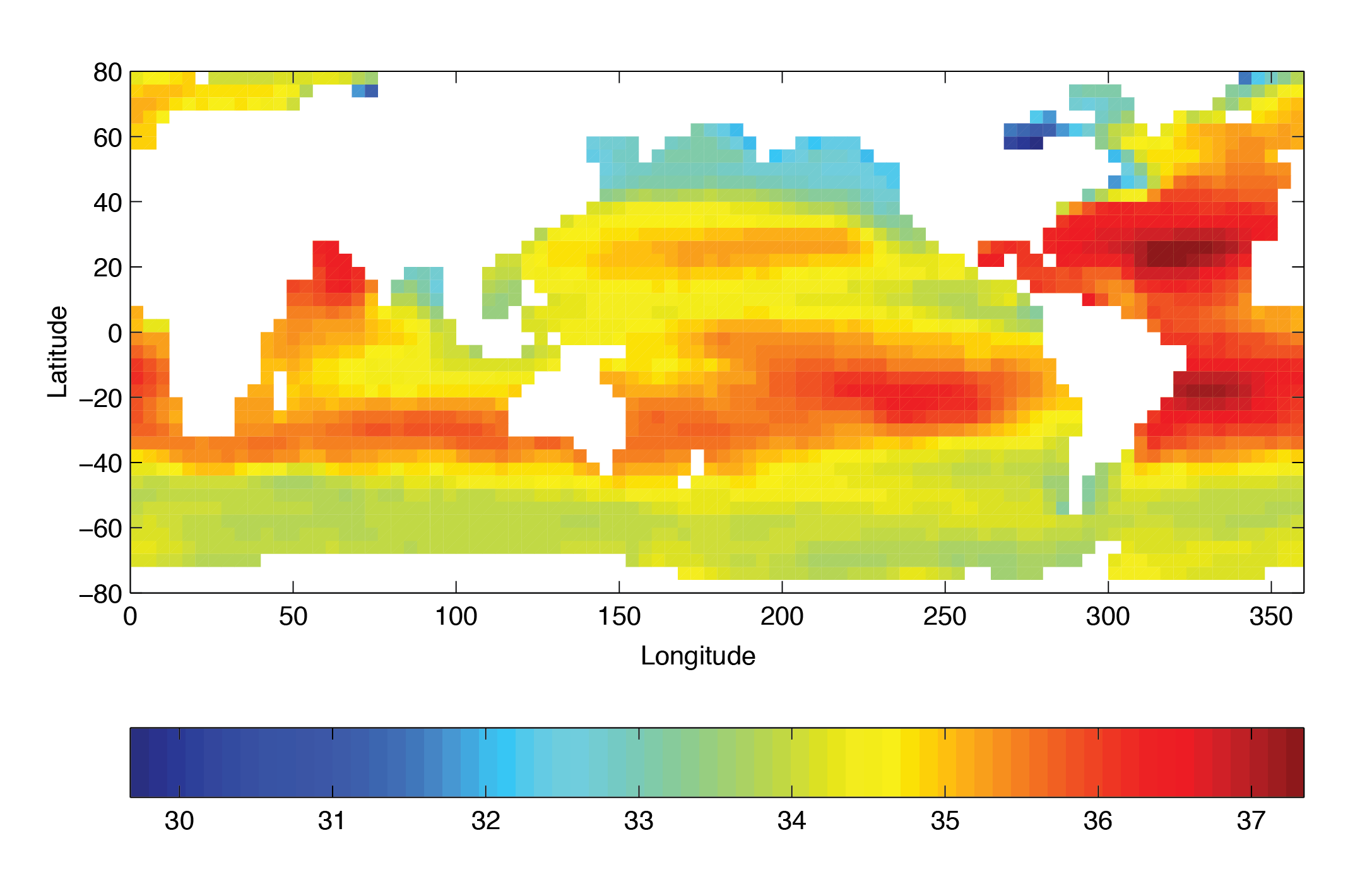
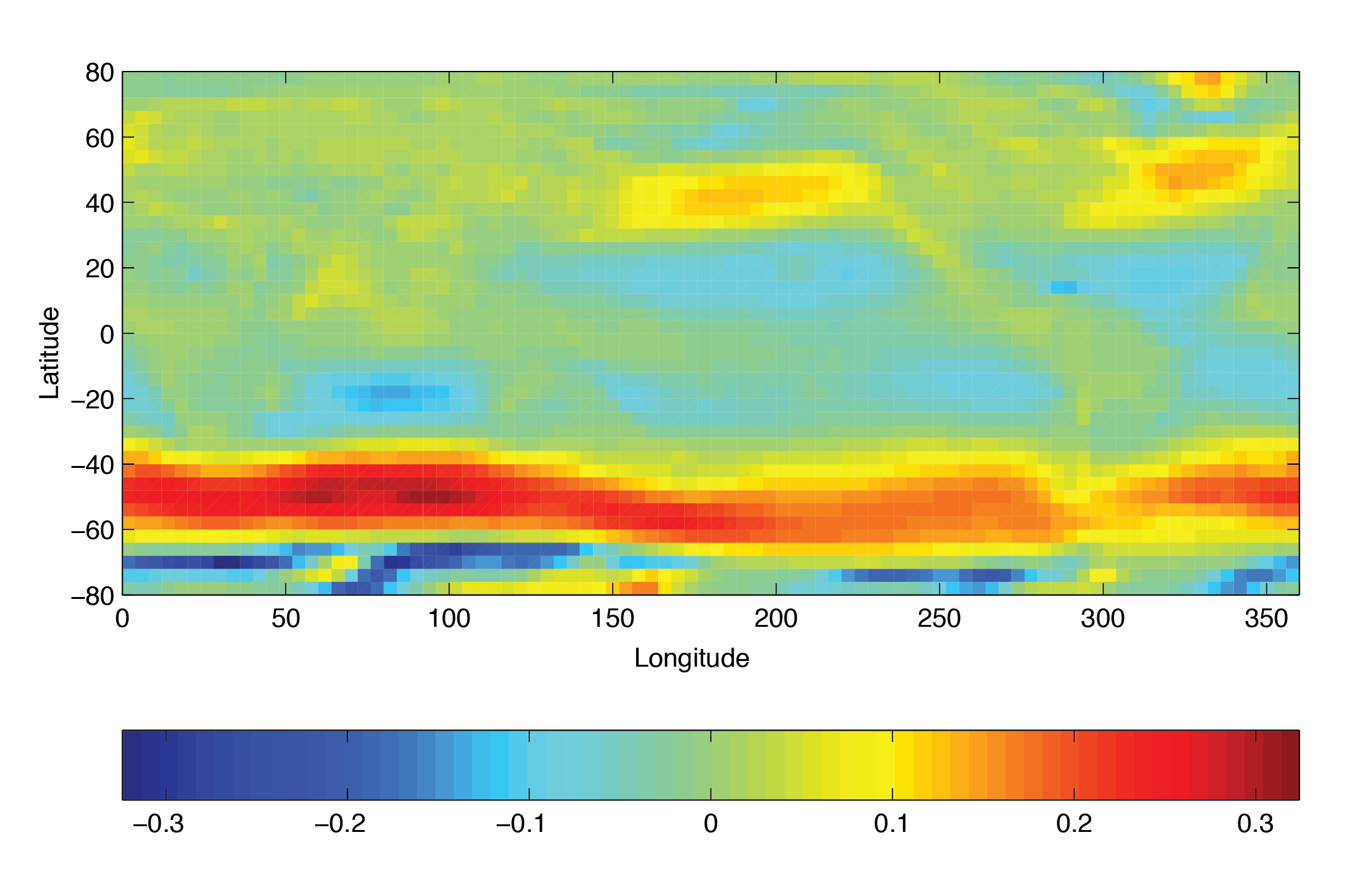
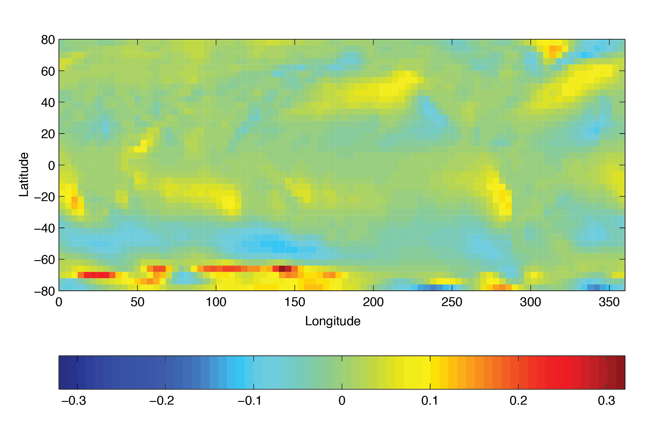
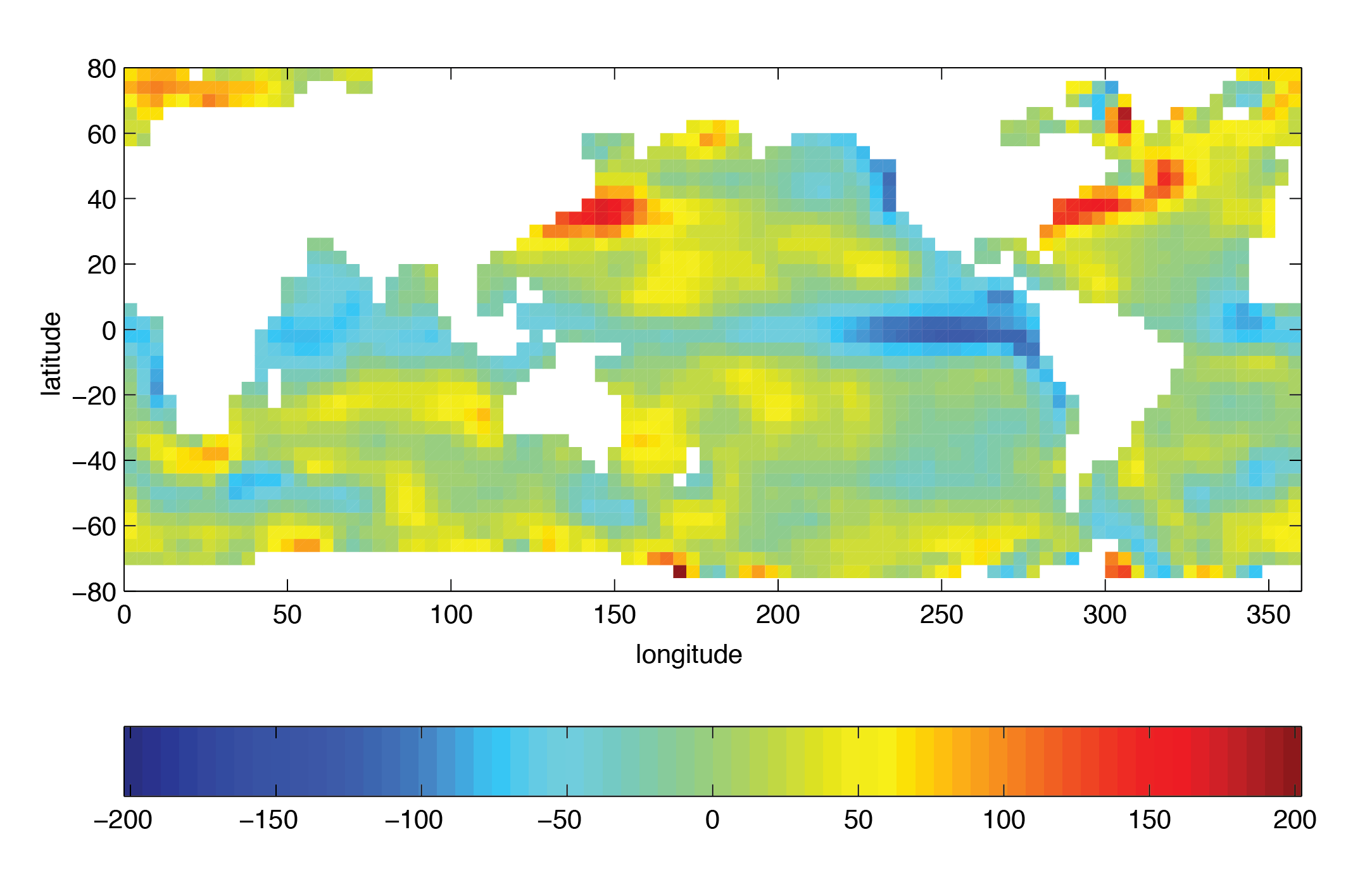
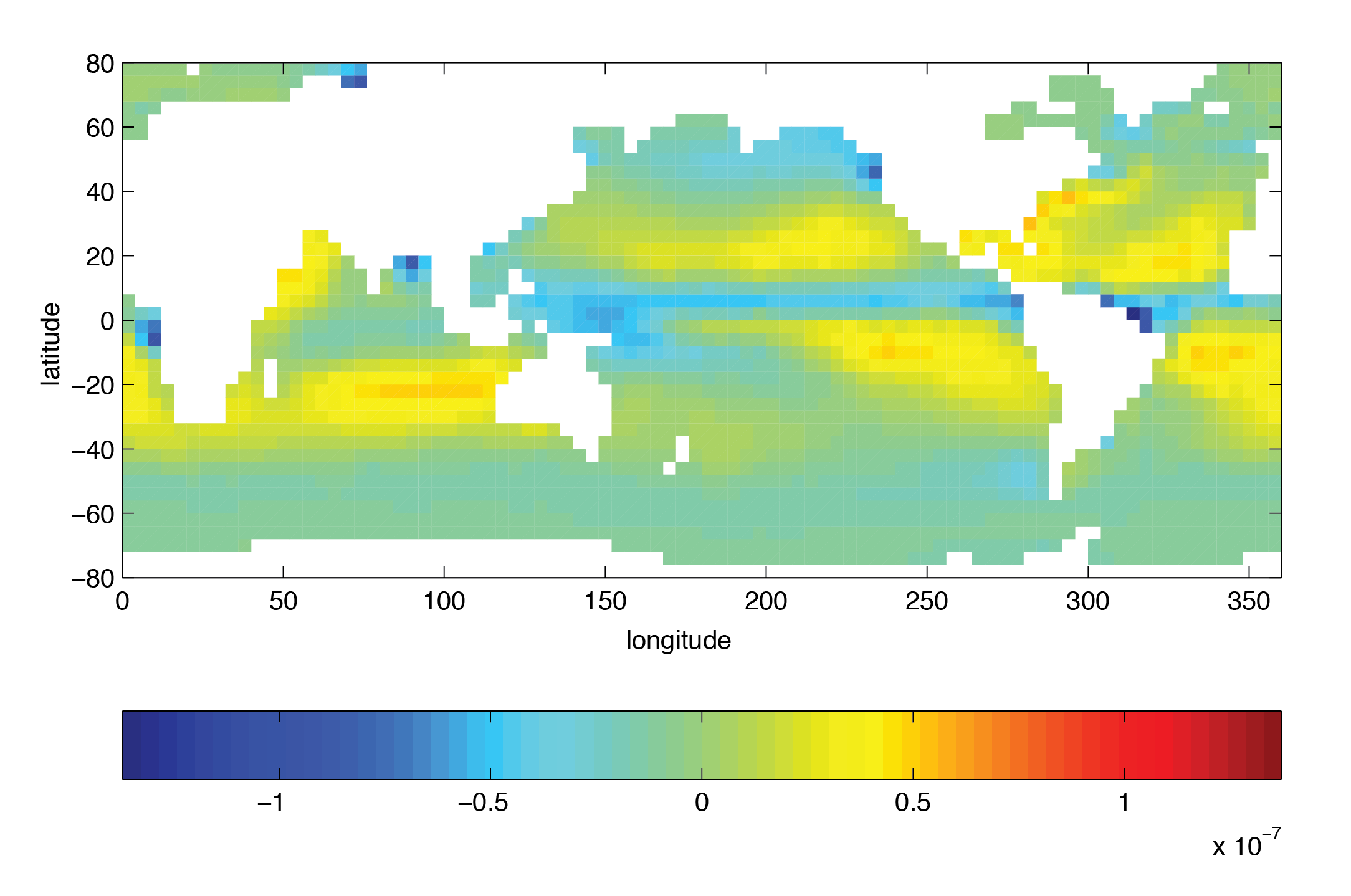
Figure 4.26-Figure 4.31
show the relaxation temperature (\(\theta^{\ast}\)) and salinity
(\(S^{\ast}\)) fields, the wind stress components (\(\tau_x\)
and \(\tau_y\)), the heat flux (\(Q\)) and the net fresh water
flux (\({\cal E} - {\cal P} - {\cal R}\)) used in equations
(4.30)-(4.33).
The figures also indicate the lateral extent and coastline used in the
experiment. Figure (— missing figure — ) shows the depth contours of
the model domain.
Figure 4.26 Annual mean of relaxation temperature (oC)
Figure 4.27 Annual mean of relaxation salinity (g/kg)
Figure 4.28 Annual mean of zonal wind stress component (N m-2)
Figure 4.29 Annual mean of meridional wind stress component (N m-2)
This file specifies the main parameters
for the experiment. The parameters that are significant for this
configuration are
Lines 7-8,
tRef= 15*20.,
sRef= 15*35.,
set reference values for potential temperature and salinity at each
model level in units of oC and
ppt. The entries are ordered from surface to depth.
Density is calculated from anomalies at each level evaluated with
respect to the reference values set here.
Line 9,
viscAr=1.E-3,
this line sets the vertical Laplacian dissipation coefficient to
\(1 \times 10^{-3}\) m2 s-1. Boundary conditions for
this operator are specified later.
Line 10,
viscAh=5.E5,
this line sets the horizontal Laplacian frictional dissipation
coefficient to \(5 \times 10^{5}\) m2 s-1. Boundary
conditions for this operator are specified later.
Lines 11, 13,
diffKhT=0.,
diffKhS=0.,
set the horizontal diffusion coefficient for temperature and salinity
to 0, since pkg/gmredi is used.
Lines 12, 14,
diffKrT=3.E-5,
diffKrS=3.E-5,
set the vertical diffusion coefficient for temperature and salinity
to \(3 \times 10^{-5}\) m2 s-1. The boundary
condition on this operator is \(\frac{\partial}{\partial z}=0\)
at both the upper and lower boundaries.
set the reference densities for sea water and fresh water, and
selects the equation of state (Jackett and McDougall 1995 [JM95])
Lines 18-19,
ivdc_kappa=100.,
implicitDiffusion=.TRUE.,
specify an “implicit diffusion” scheme with increased vertical
diffusivity of 100 m2/s in case of instable
stratification.
Line 28,
readBinaryPrec=32,
Sets format for reading binary input datasets containing model fields
to use 32-bit representation for floating-point numbers.
Line 33,
cg2dMaxIters=500,
Sets maximum number of iterations the two-dimensional, conjugate
gradient solver will use, irrespective of convergence criteria
being met.
Line 34,
cg2dTargetResidual=1.E-13,
Sets the tolerance which the 2-D conjugate gradient
solver will use to test for convergence in
(2.15) to \(1 \times 10^{-13}\).
Solver will iterate until tolerance falls below this value or until
the maximum number of solver iterations is reached.
Line 39,
nIter0=0,
Sets the starting time for the model internal time counter. When set
to non-zero this option implicitly requests a checkpoint file be read
for initial state. By default the checkpoint file is named according
to the integer number of time step value nIter0. The internal
time counter works in seconds. Alternatively, startTime can be
set.
Line 40,
nTimeSteps=20,
Sets the time step number at which this simulation will terminate. At
the end of a simulation a checkpoint file is automatically written so
that a numerical experiment can consist of multiple stages.
Alternatively endTime can be set.
Line 44,
deltaTmom=1800.,
Sets the timestep \(\Delta t_{v}\) used in the momentum equations
to 30 minutes. See Section 2.2.
Line 45,
tauCD=321428.,
Sets the D-grid to C-grid coupling time scale \(\tau_{CD}\) used
in the momentum equations.
Sets the default timestep, \(\Delta t_{\theta}\), for tracer
equations and implicit free surface equations to
24 hours. See Section 2.2.
Line 76,
bathyFile='bathymetry.bin'
This line specifies the name of the file from which the domain
bathymetry is read. This file is a 2-D (\(x,y\)) map
of depths. This file is assumed to contain 32-bit binary numbers
giving the depth of the model at each grid cell, ordered with the \(x\)
coordinate varying fastest. The points are ordered from low
coordinate to high coordinate for both axes. The units and
orientation of the depths in this file are the same as used in the
MITgcm code. In this experiment, a depth of 0 m indicates a
solid wall and a depth of <0 m indicates open ocean.
These lines specify the names of the files from which the \(x\)- and \(y\)-
direction surface wind stress is read. These files are also
3-D (\(x,y,time\)) maps and are enumerated and
formatted in the same manner as the bathymetry file.
Other lines in the file input/data
are standard values that are described in the Section 3.8.
This file uses standard default values and does not contain
customizations for this experiment.
4.5.3.5. Files input/trenberth_taux.bin and input/trenberth_tauy.bin
The input/trenberth_taux.bin and input/trenberth_tauy.bin files
specify 3-D (\(x,y,time\)) maps of wind stress
\((\tau_{x},\tau_{y})\), based on values from Treberth et al. (1990) [TOL90].
The units are N m-2.
The input/bathymetry.bin file specifies a 2-D
(\(x,y\)) map of depth values. For this experiment values range
between 0 and -5200 m, and have been derived
from ETOPO5. The file contains a raw binary stream of data that is
enumerated in the same way as standard MITgcm 2-D horizontal arrays.
1CBOP
2C !ROUTINE: SIZE.h
3C !INTERFACE:
4C include SIZE.h
5C !DESCRIPTION: \bv
6C *==========================================================*
7C | SIZE.h Declare size of underlying computational grid.
8C *==========================================================*
9C | The design here supports a three-dimensional model grid
10C | with indices I,J and K. The three-dimensional domain
11C | is comprised of nPx*nSx blocks (or tiles) of size sNx
12C | along the first (left-most index) axis, nPy*nSy blocks
13C | of size sNy along the second axis and one block of size
14C | Nr along the vertical (third) axis.
15C | Blocks/tiles have overlap regions of size OLx and OLy
16C | along the dimensions that are subdivided.
17C *==========================================================*
18C \ev
19C
20C Voodoo numbers controlling data layout:
21C sNx :: Number of X points in tile.
22C sNy :: Number of Y points in tile.
23C OLx :: Tile overlap extent in X.
24C OLy :: Tile overlap extent in Y.
25C nSx :: Number of tiles per process in X.
26C nSy :: Number of tiles per process in Y.
27C nPx :: Number of processes to use in X.
28C nPy :: Number of processes to use in Y.
29C Nx :: Number of points in X for the full domain.
30C Ny :: Number of points in Y for the full domain.
31C Nr :: Number of points in vertical direction.
32CEOP
33 INTEGER sNx
34 INTEGER sNy
35 INTEGER OLx
36 INTEGER OLy
37 INTEGER nSx
38 INTEGER nSy
39 INTEGER nPx
40 INTEGER nPy
41 INTEGER Nx
42 INTEGER Ny
43 INTEGER Nr
44 PARAMETER (
45 & sNx = 45,
46 & sNy = 40,
47 & OLx = 2,
48 & OLy = 2,
49 & nSx = 2,
50 & nSy = 1,
51 & nPx = 1,
52 & nPy = 1,
53 & Nx = sNx*nSx*nPx,
54 & Ny = sNy*nSy*nPy,
55 & Nr = 15)
5657C MAX_OLX :: Set to the maximum overlap region size of any array
58C MAX_OLY that will be exchanged. Controls the sizing of exch
59C routine buffers.
60 INTEGER MAX_OLX
61 INTEGER MAX_OLY
62 PARAMETER ( MAX_OLX = OLx,
63 & MAX_OLY = OLy )
64
Four lines are customized in this file for the current experiment
Line 45,
sNx=45,
this line sets the number of grid points of each tile (or sub-domain)
along the \(x\)-coordinate axis.
Line 46,
sNy=40,
this line sets the number of grid points of each tile (or sub-domain)
along the \(y\)-coordinate axis.
Lines 49,51,
nSx=2,
nPx=1,
these lines set, respectively, the number of tiles per process and the number of processes
along the \(x\)-coordinate axis. Therefore,
the total number of grid points along the \(x\)-coordinate axis
corresponding to the full domain extent is \(Nx=sNx*nSx*nPx=90\).
Line 55,
Nr=15
this line sets the vertical domain extent in grid points.