This example experiment demonstrates using the MITgcm to simulate a barotropic, wind-forced, ocean gyre circulation.
The experiment is a numerical rendition of the gyre circulation problem described analytically
by Stommel in 1948 [Sto48] and Munk in 1950 [Mun50], and numerically in Bryan (1963) [Bry63].
Note this tutorial assumes a basic familiarity with ocean dynamics and geophysical fluid dynamics; readers new to the field
may which to consult one of the standard texts on these subjects,
such as Vallis (2017) [Val17] or Cushman-Roisin and Beckers (2011) [CRB11].
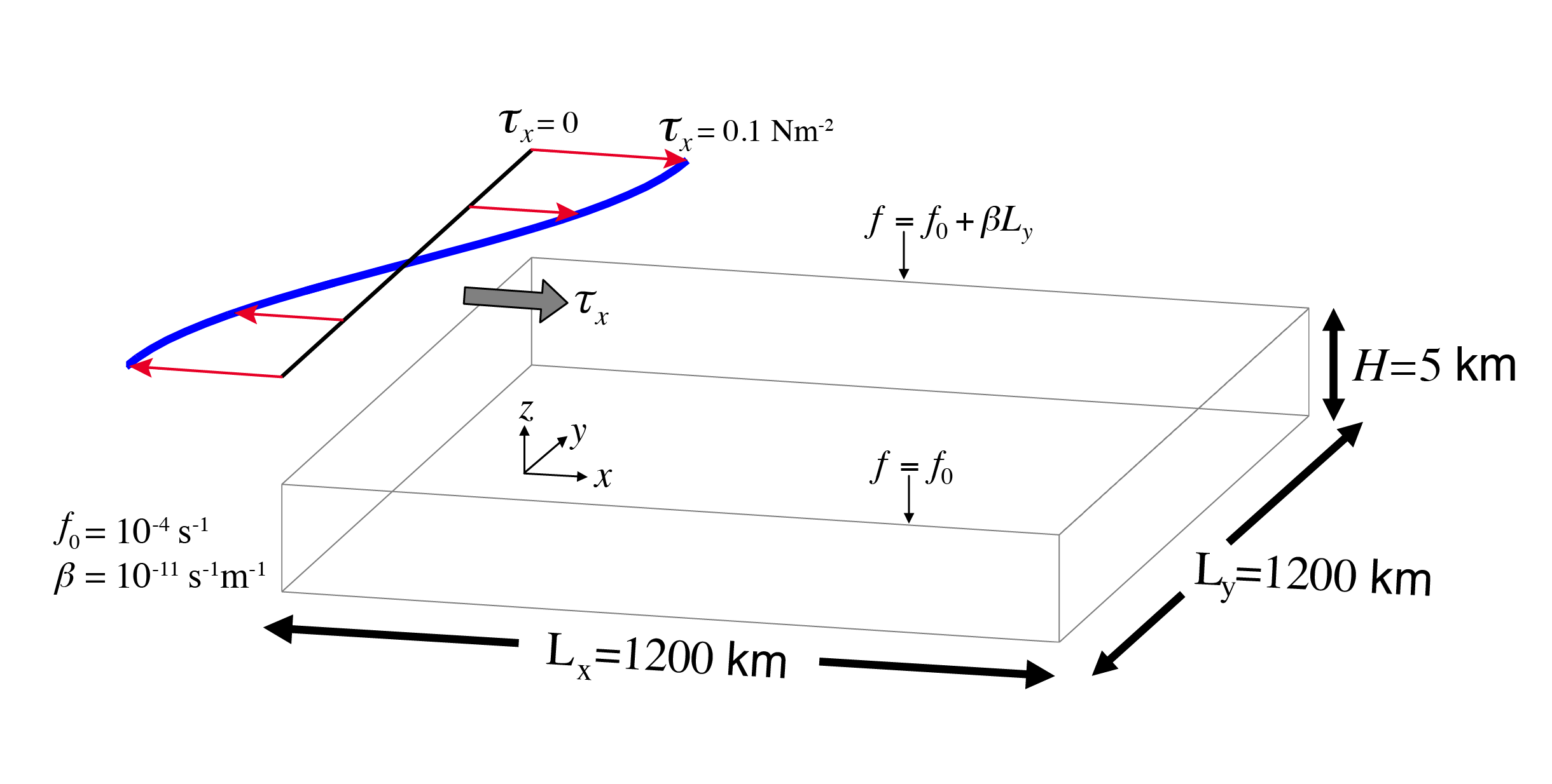
In this experiment the model is configured to represent a rectangular enclosed box of fluid, \(1200 \times 1200\) km
in lateral extent. The fluid depth \(H =\) 5 km. The fluid is forced by a zonal wind stress, \(\tau_x\), that varies
sinusoidally in the north-south direction and is constant in time. Topologically the grid is Cartesian and the Coriolis parameter \(f\) is
defined according to a mid-latitude beta-plane equation
\[f(y) = f_{0}+\beta y\]
where \(y\) is the distance along the ‘north-south’ axis of the simulated domain. For this experiment \(f_{0}\) is
set to \(10^{-4}\text{s}^{-1}\) and \(\beta = 10^{-11}\text{s}^{-1}\text{m}^{-1}\).
The sinusoidal wind-stress variations are defined according to
where \(L_{y}\) is the lateral domain extent and
\(\tau_0\) is set to \(0.1 \text{N m}^{-2}\).
Figure 4.1 summarizes the configuration simulated.
Figure 4.1 Schematic of simulation domain and wind-stress forcing function for barotropic gyre numerical experiment. The domain is enclosed by solid walls at \(x=\) 0, 1200 km and at \(y=\) 0, 1200 km.
The model is configured in hydrostatic form (the MITgcm default). The implicit free surface form of the
pressure equation described in Marshall et al. (1997) [MHPA97] is employed.
A horizontal Laplacian operator \(\nabla_{h}^2\) provides viscous
dissipation. The wind-stress momentum input is added to the momentum equation
for the ‘zonal flow’, \(u\). This effectively yields an active set of
equations for this configuration as follows:
where \(u\) and \(v\) are the \(x\) and \(y\) components of the
flow vector \(\vec{\bf u}\), \(\eta\) is the free surface height,
\(A_{h}\) the horizontal Laplacian viscosity, \(\rho_{c}\) is the fluid density,
and \(g\) the acceleration due to gravity.
The domain is discretized with a uniform grid spacing in the horizontal set to \(\Delta x=\Delta y=20\) km,
so that there are sixty ocean grid cells in the \(x\) and \(y\) directions. The numerical
domain includes a border row of “land” cell surrounding the ocean cells, so the numerical grid size is 62\(\times\)62
(if these land cells were not included, the domain would be periodic in both
the \(x\) and \(y\) directions).
Vertically the model is configured using a single layer in depth, \(\Delta z\), of 5000 m.
Let’s start with our choice for the model’s time step. To minimize the amount of required computational resources, typically one
opts for as large a time step as possible while keeping the model solution stable. The advective
Courant–Friedrichs–Lewy (CFL) condition (see Adcroft 1995 [Adc95]) for an extreme
maximum horizontal flow speed is:
The 2 factor on the left is because we have a 2-D problem
(in contrast with the more familiar 1-D canonical stability analysis); the right hand side is 0.5
due to our default use of Adams-Bashforth2 (see Section 2.5) rather than the more familiar
value of 1 that one would obtain using a forward Euler scheme.
In our configuration, let’s assume our solution will achieve a maximum \(| u | = 1\) ms–1
(in reality, current speeds in our solution will be much smaller). To keep \(\Delta t\) safely
below the stability threshold, let’s choose \(\Delta t\) = 1200 s (= 20 minutes), which
results in \(S_{\rm adv}\) = 0.12.
The numerical stability for inertial oscillations using Adams-Bashforth II (Adcroft 1995 [Adc95])
(4.5)\[S_{\rm inert} = f {\Delta t} < 0.5 \text{ for stability}\]
evaluates to 0.12 for our choice of \(\Delta t\), which is below the stability threshold.
There are two general rules in choosing a horizontal Laplacian eddy viscosity \(A_{h}\):
the resulting Munk layer width should be at least as large (preferably, larger) than the lateral grid spacing;
the viscosity should be sufficiently small that the model is stable for horizontal friction, given the time step.
Let’s use this first rule to make our choice for \(A_{h}\), and check this value using the second rule.
The theoretical Munk boundary layer width (as defined by the solution
zero-crossing, see Pedlosky 1987 [Ped87]) is given by:
For our configuration we will choose to resolve a boundary layer of \(\approx\) 100 km,
or roughly across five grid cells, so we set \(A_{h} = 400\) m2 s–1
(more precisely, this sets the full width at \(M\) = 124 km). This choice ensures
that the frictional boundary layer is well resolved.
Given our choice of \(\Delta t\), the stability
parameter for the horizontal Laplacian friction (Adcroft 1995 [Adc95])
evaluates to 0.0096, which is well below the stability threshold. As in (4.4) the above criteria
is for a 2D problem using Adams-Bashforth2 time stepping, with the 0.6 value on the right replacing the more familiar 1
that is obtained using a forward Euler scheme.
See Section 2.5 for additional details on Adams-Bashforth time-stepping and numerical stability criteria.
contain the code customizations and parameter settings for this
experiment. Below we describe these customizations in detail.
Note: MITgcm’s defaults are configured to simulate an ocean rather than an atmosphere, with vertical \(z\)-coordinates.
To model the ocean using pressure coordinates using MITgcm, additional parameter changes are required; see tutorial ocean_in_p.
To switch parameters to model an atmosphere, see tutorial Held_Suarez.
1CBOP
2C !ROUTINE: SIZE.h
3C !INTERFACE:
4C include SIZE.h
5C !DESCRIPTION: \bv
6C *==========================================================*
7C | SIZE.h Declare size of underlying computational grid.
8C *==========================================================*
9C | The design here supports a three-dimensional model grid
10C | with indices I,J and K. The three-dimensional domain
11C | is comprised of nPx*nSx blocks (or tiles) of size sNx
12C | along the first (left-most index) axis, nPy*nSy blocks
13C | of size sNy along the second axis and one block of size
14C | Nr along the vertical (third) axis.
15C | Blocks/tiles have overlap regions of size OLx and OLy
16C | along the dimensions that are subdivided.
17C *==========================================================*
18C \ev
19C
20C Voodoo numbers controlling data layout:
21C sNx :: Number of X points in tile.
22C sNy :: Number of Y points in tile.
23C OLx :: Tile overlap extent in X.
24C OLy :: Tile overlap extent in Y.
25C nSx :: Number of tiles per process in X.
26C nSy :: Number of tiles per process in Y.
27C nPx :: Number of processes to use in X.
28C nPy :: Number of processes to use in Y.
29C Nx :: Number of points in X for the full domain.
30C Ny :: Number of points in Y for the full domain.
31C Nr :: Number of points in vertical direction.
32CEOP
33 INTEGER sNx
34 INTEGER sNy
35 INTEGER OLx
36 INTEGER OLy
37 INTEGER nSx
38 INTEGER nSy
39 INTEGER nPx
40 INTEGER nPy
41 INTEGER Nx
42 INTEGER Ny
43 INTEGER Nr
44 PARAMETER (
45     &           sNx =  62,
46     &           sNy =  62,
47     &           OLx =   2,
48     &           OLy =   2,
49     &           nSx =   1,
50     &           nSy =   1,
51     &           nPx =   1,
52     &           nPy =   1,
53     &           Nx  = sNx*nSx*nPx,
54     &           Ny  = sNy*nSy*nPy,
55 & Nr = 1)
5657C MAX_OLX :: Set to the maximum overlap region size of any array
58C MAX_OLY that will be exchanged. Controls the sizing of exch
59C routine buffers.
60 INTEGER MAX_OLX
61 INTEGER MAX_OLY
62 PARAMETER ( MAX_OLX = OLx,
63 & MAX_OLY = OLy )
64
Here we show a modified model/inc source code file, customizing MITgcm’s array sizes to our model domain.
This file must be uniquely configured for any model setup; using the MITgcm default
model/inc/SIZE.h will in fact cause a compilation error.
Note that MITgcm’s storage arrays are allocated as static variables
(hence their size must be declared in the source code), in contrast to some model codes which declare array sizes dynamically,
i.e., through runtime (namelist) parameter settings.
For this first tutorial, our setup and run environment is the most simple possible: we run on a single process
(i.e., NOT MPI and NOT multi-threaded)
using a single model “tile”. For a more complete explanation of the parameter choices to use multiple tiles,
see the tutorial Baroclinic Gyre.
These lines set parameters sNx and sNy, the number of grid points in the \(x\) and \(y\) directions, respectively.
45 & sNx = 62,
46 & sNy = 62,
These lines set parameters OLx and OLy in the \(x\) and \(y\) directions, respectively.
These values are the overlap extent of a model tile, the purpose of which will be explained in later tutorials.
Here, we simply specify the required minimum value (2)
in both \(x\) and \(y\).
47 & OLx = 2,
48 & OLy = 2,
These lines set parameters nSx, nSy, nPx, and nPy,
the number of model tiles and the number of processes in the \(x\) and \(y\) directions, respectively.
As discussed above, in this tutorial we configure a single model tile on
a single process, so these parameters are all set to the value one.
This file, reproduced completely above, specifies the main parameters
for the experiment. The parameters that are significant for this configuration
(shown with line numbers to left) are as follows.
This line sets parameter viscAh, the horizontal Laplacian viscosity, to \(400\) m2 s–1.
4 viscAh=4.E2,
These lines set \(f_0\) and \(\beta\) (the Coriolis parameter f0 and
the gradient of the Coriolis parameter beta) for our beta-plane to
\(1 \times 10^{-4}\) s–1 and \(1 \times 10^{-11}\) m–1s–1, respectively.
5 f0=1.E-4,
6 beta=1.E-11,
This line sets parameter rhoConst, the Boussinesq reference density
\(\rho_c\) in (4.1), to 1000 kg/m3.
7 rhoConst=1000.,
This line sets parameter gBaro, the acceleration due to gravity \(g\) (in the free surface terms
in (4.1) and (4.2)), to 9.81 m/s2.
This is the MITgcm default value, i.e., the value used if this line were not
included in data. One might alter this parameter for a reduced gravity model, or to simulate a different planet, for example.
8 gBaro=9.81,
These lines set parameters rigidLid and implicitFreeSurface in order to
suppress the rigid lid formulation of the surface pressure inverter and activate the implicit free surface formulation.
This line sets parameter momAdvection to suppress the (non-linear) momentum of advection
terms in the momentum equations. However, note the # in column 1: this
“comments out” the line, so using the above data
file verbatim will in fact include the momentum advection terms (i.e., MITgcm default for this parameter is TRUE).
We’ll explore the linearized solution (i.e., by removing the leading #) in Section 4.1.5.
Note the ability to comment out a line in a namelist file is not part of standard Fortran,
but this feature is implemented for all MITgcm namelist files.
11# momAdvection=.FALSE.,
These lines set parameters tempStepping and saltStepping to
suppress MITgcm’s forward time integration of temperature and salt in the tracer equations,
as these prognostic variables are not relevant for the model solution in this configuration.
By default, MITgcm solves equations governing these two (active) tracers; later tutorials will
demonstrate how additional passive tracers can be included in the solution.
The advantage of NOT solving the temperature and salinity equations is to
eliminate many unnecessary computations. In most typical configurations however, one will want the model to
compute a solution for \(T\) and \(S\), which
typically comprises the majority of MITgcm’s processing time.
The first line sets the tolerance (parameter cg2dTargetResidual) that the 2-D conjugate gradient solver,
the iterative method used in the pressure method algorithm, will use to test for convergence.
The second line sets parameter cg2dMaxIters, the maximum
number of iterations.
The solver will iterate until the residual falls below this target value
(here, set to \(1 \times 10^{-7}\)) or until this maximum number of solver iterations is reached
(here, set to a maximum 1000 iterations). Typically, the solver will converge in far fewer than 1000 iterations, but
it does not hurt to allow for a large number. The chosen value for the target residual
happens to be the MITgcm default, and will serve well
in most model configurations.
This line sets the starting (integer) iteration number for the run. Here we set the value to zero, which starts the model from a new, initialized state.
If nIter0 is non-zero, the model would require appropriate pickup files (i.e., restart files) in order to continue integration of an existing run.
24 nIter0=0,
This line sets parameter nTimeSteps, the (integer) number of timesteps the model will integrate forward. Below,
we have set this to integrate for just 10 time steps, for MITgcm automated testing purposes (Section 5.5).
To integrate the solution to near steady state,
uncomment the line further down where we set the value to 77760 time steps. When you make this change,
be sure to also uncomment the next line that sets monitorFreq (see below).
25 nTimeSteps=10,
32#-for longer run (3.0 yr):
33# nTimeSteps=77760,
34# monitorFreq=864000.,
This line sets parameter deltaT, the timestep used in stepping forward the model, to 1200 seconds.
In combination with the larger value of nTimeSteps mentioned above,
we have effectively set the model to integrate forward for \(77760 \times 1200 \text{ s} = 3.0\) years (based on 360-day years), long enough for the solution to approach equilibrium.
26 deltaT=1200.0,
These lines control the frequency at which restart (a.k.a. pickup) files are dumped by MITgcm.
Here the value of pChkptFreq is set to 31,104,000 seconds (=1.0 years) of model time;
this controls the frequency of “permanent” checkpoint pickup files. With permanent files,
the model’s iteration number is part of the file name (as the filename “suffix”; see Section 4.1.4.2)
in order to save it as a labelled, permanent, pickup state.
The value of ChkptFreq is set to 15,552,000 seconds (=0.5 years); the pickup files
written at this frequency but will NOT include the iteration number in the filename,
instead toggling between ckptA and ckptB in the filename, and thus these
files will be overwritten with new data every 2 \(\times\) 15,552,000 seconds.
Temporary checkpoint files can be written more frequently without requiring additional disk space,
for example to peruse (or re-run) the model state prior to an instability,
or restart following a computer crash, etc.
Either type of checkpoint file can be used to restart the model.
This line sets parameter dumpFreq, frequency of writing model state
snapshot diagnostics (of relevance in this setup: variables \(u\), \(v\), and \(\eta\)).
Here, we opt for a snapshot of model state every 15,552,000 seconds (=0.5 years), or after every 12960 time steps of integration.
29 dumpFreq=15552000.0,
These lines are set to dump monitor output (see Section 9.4) every 1200 seconds (i.e., every time step) to standard output.
While this monitor frequency is needed for MITgcm automated testing, this is too much output for our tutorial run. Comment out this line
and uncomment the line where monitorFreq is set to 864,000 seconds, i.e., output every 10 days.
Parameter monitorSelect is set to 2 here to reduce output of non-applicable quantities for this simple example.
This line sets parameter usingCartesianGrid, which specifies that the simulation will use a Cartesian coordinate system.
39 usingCartesianGrid=.TRUE.,
These lines set the horizontal grid spacing of the model grid, as vectors delX and delY
(i.e., \(\Delta x\) and \(\Delta y\) respectively).
This syntax indicates that we specify 62 values in both the \(x\) and \(y\) directions, which matches the
domain size as specified in SIZE.h.
Grid spacing is set to \(20 \times 10^{3}\) m (=20 km).
40 delX=62*20.E3,
41 delY=62*20.E3,
The cartesian grid default origin is (0,0) so here we set the origin with
parameters xgOrigin and ygOrigin to (-20000,-20000),
accounting for the bordering solid wall.
The centers of the grid boxes will thus be at -10 km, 10 km, 30 km, 50 km, …,
in both \(x\) and \(y\) directions.
42 xgOrigin=-20.E3,
43 ygOrigin=-20.E3,
This line sets parameter delR, the vertical grid spacing in the \(z\)-coordinate (i.e., \(\Delta z\)), to 5000 m.
This line sets parameter bathyFile, the name of the bathymetry file.
See Section 4.1.3.2.4 for information about the file format.
49 bathyFile='bathy.bin'
These lines specify the names of the files from which the surface wind stress is read.
There is a separate file for the \(x\)-direction (zonalWindFile) and the \(y\)-direction (meridWindFile).
Note, here we have left the latter parameter blank, as there is no meridional wind stress forcing in our example.
This file does not set any namelist parameters, yet is necessary to run – only standard packages
(i.e., those compiled in MITgcm by default) are required for this setup, so no other customization is necessary.
We will demonstrate how to include additional packages
in other tutorial experiments.
 1# Example "eedata" file
 2# Lines beginning "#" are comments
 3#  nTx      :: No. threads per process in X
 4#  nTy      :: No. threads per process in Y
 5# debugMode :: print debug msg (sequence of S/R calls)
 6 &EEPARMS
 7 nTx=1,
 8 nTy=1,
 9 &
10# Note: Some systems use & as the namelist terminator (as shown here).
11#       Other systems use a / character.
This file uses standard default values (i.e., MITgcm default is single-threaded) and does not contain
customizations for this experiment.
This file is a 2-D(\(x,y\)) map of bottom bathymetry, specified as the \(z\)-coordinate of the solid bottom boundary.
Here, the value is set to -5000 m everywhere except along the N, S, E, and W edges of the array, where the
value is set to 0 (i.e., “land”). As discussed in Section 4.1.2, the domain in MITgcm is assumed doubly periodic
(i.e., periodic in both \(x\)- and \(y\)-directions), so boundary walls
are necessary to set up our enclosed box domain.
The matlab program verification/tutorial_barotropic_gyre/input/gendata.m
was used to generate this bathymetry file (alternatively, see python equivalent
gendata.py). By default, this file is assumed to
contain 32-bit (single precision) binary numbers.
See Section 3.9 for additional information on MITgcm input data file format specifications.
Similar to file input/bathy.bin, this file is a 2-D(\(x,y\))
map of \(\tau_{x}\) wind stress values, formatted in the same manner.
The units are Nm–2. Although \(\tau_{x}\) is only a function of \(y\) in this experiment,
this file must still define a complete 2-D map in order
to be compatible with the standard code for loading forcing fields
in MITgcm. The matlab program verification/tutorial_barotropic_gyre/input/gendata.m
was used to generate this wind stress file (alternatively, see python equivalent
gendata.py).
To run the barotropic jet variation of this tutorial example (see Figure 4.4),
you will in fact need to run one of these
programs to generate the file input/windx_siny.bin.
Your run’s standard output file should be similar to verification/tutorial_barotropic_gyre/results/output.txt.
The standard output is essentially a log file of the model run. The following information is included (in rough order):
startup information including MITgcm checkpoint release number and other execution environment information,
and a list of activated packages (including all default packages, as well as optional packages).
the text from all data.* and other critical files (in our example here,
eedata,
SIZE.h,
data,
and data.pkg).
information about the grid and bathymetry, including dumps of all grid variables (only if Cartesian or spherical polar coordinates used, as is the case here).
all runtime parameter choices used by the model, including all model defaults as well as user-specified parameters.
monitor statistics at regular intervals (as specified by parameter
monitorFreq in data. See Section 9.4).
output from the 2-D conjugate gradient solver. More specifically, statistics from the right-hand side of the elliptic
equation – for our linear free-surface, see eq. (2.15) – are dumped for every model time step. If the model solution
blows up, these statistics will increase to infinity, so one can see exactly when the problem occurred (i.e., to aid in debugging). Additional
solver variables, such as number of iterations and residual, are included with the monitor statistics.
a summary of end-of-run execution information, including user-, wall- and system-time elapsed during execution,
and tile communication statistics.
These statistics are provided for the overall run, and also broken down by time spent in various subroutines.
Different setups using non-standard packages and/or different parameter choices will include
additional or different output as part of the standard output. It is also possible to select more or less output
by changing the parameter debugLevel in data; see (missing doc for pkg debug).
STDERR.0000 - if errors (or warnings) occurred during the run, helpful warning and/or error message(s) would appear in this file.
In addition to raw binary data files with .data extension, each binary file has a corresponding .meta file. These plain-text files include
information about the array size, precision (i.e., float32 or float64), and if relevant, time information and/or
a list of these fields included in the binary file. The .meta files are used by MITgcm utils when binary data are read.
The following output files are generated:
Grid Data: see Section 2.11 for definitions and description of the Arakawa C-grid
staggering of model variables.
XC, YC - grid cell center point locations
XG, YG - locations of grid cell vertices
RC, RF - vertical cell center and cell faces positions
DXC, DYC - grid cell center point separations (Figure 2.8 b)
DXG, DYG - separation of grid cell vertices (Figure 2.8 a)
DRC, DRF - separation of vertical cell centers and faces, respectively
RAC, RAS, RAW, RAZ - areas of the grid “tracer cells”, “southern cells”,
“western cells” and “vorticity cells”, respectively (Figure 2.8)
hFacC, hFacS, hFacW - fractions of the grid cell in the vertical which are “open” as defined
in the center and on the southern and western boundaries, respectively.
These variables effectively contain the configuration bathymetric (or topographic) information.
Depth - bathymetry depths
All these files contain 2-D(\(x,y\)) data except RC, RF, DRC, DRF, which are 1-D(\(z\)),
and hFacC, hFacS, hFacW, which contain 3D(\(x,y,z\)) data. Units for the grid files depends on one’s choice of model grid;
here, they are all in given in meters (or \(\text{m}^2\) for areas).
All the 2-D grid data files contain .001.001 in their filename, e.g., DXC.001.001.data – this is the tile number in .XXX.YYY format.
Here, we have just a single tile in both x and y, so both tile numbers are 001.
Using multiple tiles, the default is that the local tile grid information
would be output separately for each tile (as an example, see the baroclinic gyre tutorial,
which is set up using multiple tiles), producing multiple files for each 2-D grid variable.
State Variable Snapshot Data:
Eta.0000000000.001.001.data,Eta.0000000000.001.001.meta - this is
a binary data snapshot of model dynamic variable
etaN (the free-surface height) and its meta file, respectively.
Note the tile number is included in the filename, as is the iteration number 0000000000, which is simply the time step
(the iteration number here is referred to as the “suffix” in
MITgcm parlance; there are options to change this suffix to something other than iteration number).
In other words, this is a dump of the free-surface height from the initialized state,
iteration 0; if you load up this data file,
you will see it is all zeroes. More interesting is the free-surface
height after some time steps have occurred. Snapshots are written according
to our parameter choice dumpFreq, here set to 15,552,000 seconds, which is every 12960 time steps.
We will examine the model solutions in Section 4.1.5.
The free-surface height is a 2-D(\(x,y\)) field.
Snapshot files exist for other prognostic model variables, in particular
filenames starting with U (uVel),
V (uVel), T (theta), and S (salt);
given our setup, these latter two fields
remain uniform in space and time, thus not very interesting until we
explore a baroclinic gyre setup in tutorial_baroclinic_gyre.
These are all 3-D(\(x,y,z\)) fields. The format for the file names is similar
to the free-surface height files. Also dumped are snapshots
of diagnosed vertical velocity W (wVel) (note that in non-hydrostatic
simulations, W is a fully prognostic model variable).
Checkpoint Files:
The following pickup files are generated:
pickup.0000025920.001.001.data, pickup.0000025920.001.001.meta, etc. - written at frequency set by pChkptFreq
pickup.ckptA.001.001.data, pickup.ckptA.001.001.meta, pickup.ckptB.001.001.data,
pickup.ckptB.001.001.meta - written at frequency set by ChkptFreq
Other Model Output Data: Model output related to reference density and hydrostatic pressure, in files Rhoref, PHrefC, PHrefF, PH, and PHL,
is discussed in depth here in tutorial Baroclinic Ocean Gyre (as these data are not terribly interesting in this single-layer setup).
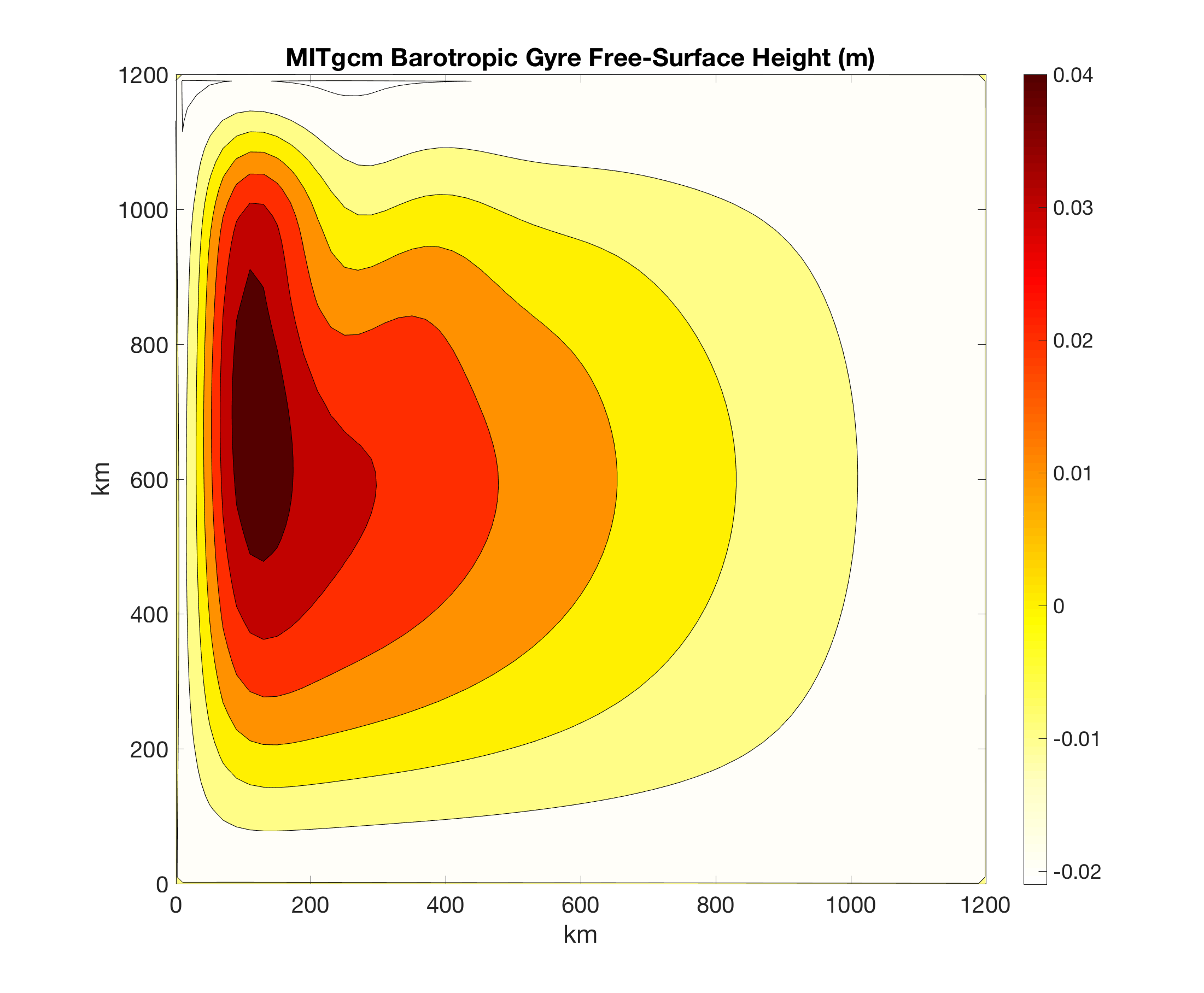
After running the model for 77,760 time steps (3.0 years), the solution is near equilibrium.
Given an approximate timescale of one month for barotropic Rossby waves
to cross our model domain, one might expect the solution to require several years to achieve an equilibrium state.
The model solution of free-surface
height \(\eta\) (proportional to streamfunction) at \(t=\) 3.0 years is shown in Figure 4.2.
For further details on this solution, particularly examining the effect of the non-linear terms with increasing Reynolds number,
the reader is referred to Pedlosky (1987) [Ped87] section 5.11.
Figure 4.2 MITgcm solution to the barotropic gyre example after \(t=\) 3.0 years of model integration. Free surface height is shown in meters.
Using matlab for example, visualizing output using the utils/matlab/rdmds.m utility to load the
binary data in Eta.0000077760.001.001.data is as simple as:
or using python (you will need to install the MITgcmutils package, see Section 11.1):
from MITgcmutils import mds
import numpy as np
import matplotlib.pyplot as plt
XC = mds.rdmds('XC')
YC = mds.rdmds('YC')
Eta = mds.rdmds('Eta', 77760)
plt.contourf(XC/1000, YC/1000, Eta, np.linspace(-0.02, 0.05,8), cmap='hot_r')
plt.colorbar()
plt.show()
(for a more involved example with detailed explanations how to read in model output,
perform calculations using these data, and make plots, see tutorial Baroclinic Ocean Gyre)
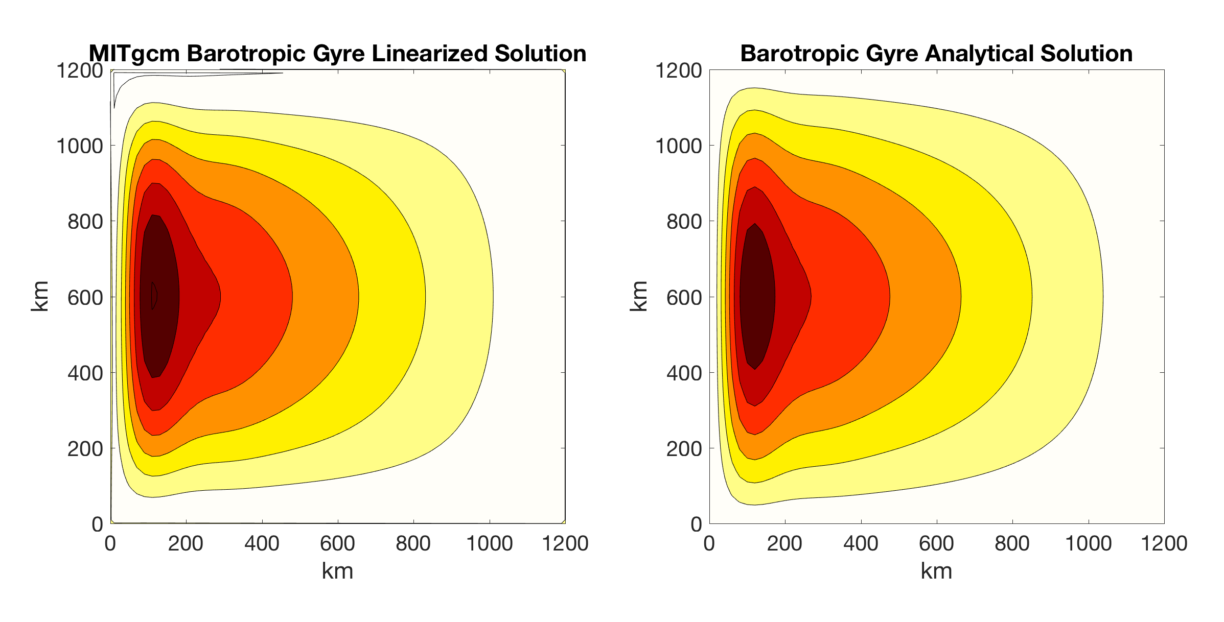
Let’s simplify the example by considering the linear problem where we neglect the advection of momentum terms.
In other words, replace \(\frac{Du}{Dt}\) and \(\frac{Dv}{Dt}\) with
\(\frac{\partial u}{\partial t}\) and \(\frac{\partial v}{\partial t}\), respectively,
in in (4.1) and (4.2).
To do so, we uncomment (i.e., remove the leading #) in the
line #momAdvection=.FALSE., in file data and re-run the model. Any existing output files will be overwritten.
For the linearized equations, the Munk layer (equilibrium) analytical solution is given by:
where \(\delta_m = (A_{h} / \beta)^{\frac{1}{3}}\). Figure 4.3
displays the MITgcm output after switching off momentum advection vs.
the analytical solution to the linearized equations. Success!
Figure 4.3 Comparison of free surface height for the near-equilibrium MITgcm solution (\(t=\) 3.0 years) with momentum advection switched off (left) and the analytical equilibrium solution to the linearized equation (right).
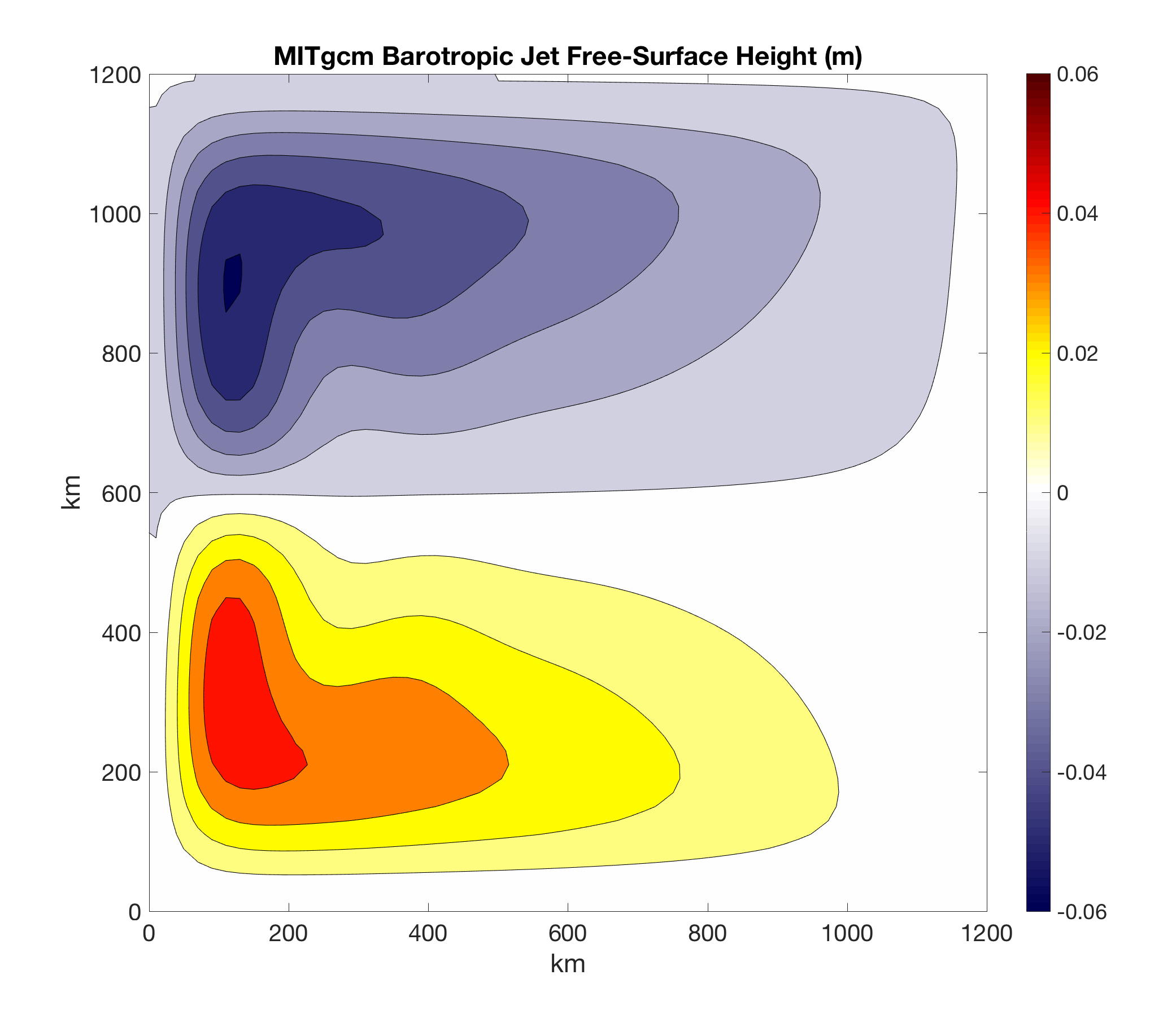
Finally, let’s examine one additional simulation where we change the cosine profile of wind stress forcing to a sine profile.
First, run the matlab script verification/tutorial_barotropic_gyre/input/gendata.m to generate the alternate sine
profile wind stress, and place a copy in your run directory. Then,
in file data,
replace the line zonalWindFile='windx_cosy.bin’, with zonalWindFile='windx_siny.bin’,.
Figure 4.4 MITgcm equilibrium solution to the barotropic setup with alternate sine profile of wind stress forcing, producing a barotropic jet.
The free surface solution given this forcing is shown in Figure 4.4. Two “half gyres” are separated by a strong jet.
We’ll look more at the solution to this “barotropic jet” setup in later tutorial examples.